Generating Unusual Molecules with Genetic Algorithms Part 2: Leveraging MolLL for Enhanced Generation

Esbenbjerrum/ April 15, 2024/ Blog/ 2 comments

In a previous blogpost: (Generating Unusual Molecules with Genetic Algorithms), I showcased the propensity of a genetic algorithm to generate unusual molecules. This illustrates that this generative algorithm needs to be kept in check. Therefore, I’ve developed a tool that appears to be capable of doing just that, based on molecular log-likelihood estimation calculated from the analysis of molecular fingerprint keys. This blog post is thus a follow-up to the previous one, and will assume that we are picking up from where we left off after creating the integrated model. To ensure self-consistency, all the necessary code from last blog-post will be included below in a single code cell.

import os
import pandas as pd
import urllib.parse
import urllib.request
from rdkit import Chem
from rdkit.Chem import Draw
from rdkit.Chem import AllChem
import numpy as np
from scipy import integrate
from sklearn.model_selection import train_test_split
from sklearn.pipeline import Pipeline
from sklearn.linear_model import Ridge
from sklearn.model_selection import GridSearchCV
import matplotlib.pyplot as plt
from scikit_mol.fingerprints import MorganFingerprintTransformer
from scikit_mol.conversions import SmilesToMolTransformer


def load_csv_from_url(url, filename=None):
    if filename is None:
        filename = os.path.basename(urllib.parse.urlsplit(url).path)
    if not os.path.isfile(filename):
        urllib.request.urlretrieve(url, filename)
    
    df = pd.read_csv(filename)
    return df

url = "https://raw.githubusercontent.com/ml-jku/mgenerators-failure-modes/master/assays/processed/CHEMBL3888429.csv"
df = load_csv_from_url(url)
df = df[~df.value.isna()] #value contains some NaN's that are filtered

def visualize_molecules_with_scores(molecule_data):
    mols = [Chem.MolFromSmiles(smiles) for _, smiles in molecule_data]
    img = Draw.MolsToGridImage(mols, molsPerRow=4, subImgSize=(200, 200), legends=[f'Score: {score:.2f}' for score, _ in molecule_data])
    return img

def plot_ga(data):
    max_values = [entry['max'] for entry in data]
    avg_values = [entry['avg'] for entry in data]
    median_values = [entry['median'] for entry in data]
    min_values = [entry['min'] for entry in data]
    std_values = [entry['std'] for entry in data]
    size_values = [entry['size'] for entry in data]
    num_func_eval_values = [entry['num_func_eval'] for entry in data]
    fig, ax1 = plt.subplots(figsize=(10, 6))
    ax1.plot(max_values, label='Max', color='blue')
    ax1.plot(avg_values, label='Avg', color='green')
    ax1.plot(median_values, label='Median', color='orange')
    ax1.fill_between(range(len(data)), min_values, max_values, color='blue', alpha=0.2)
    ax1.fill_between(range(len(data)), np.subtract(avg_values, std_values), np.add(avg_values, std_values), color='green', alpha=0.2)
    ax1.set_xlabel('Data Point')
    ax1.set_ylabel('Values')
    ax1.set_title('Max, Avg, and Median with Shaded Areas')
    ax2 = ax1.twinx()
    ax2.plot(size_values, label='Size', linestyle='--', color='red')
    ax2.plot(num_func_eval_values, label='Num Func Eval', linestyle='--', color='purple')
    ax2.set_ylabel('Size / Num Func Eval')
    ax1.legend(loc='upper left')
    ax2.legend(loc='upper right')
    return plt

def get_top_ten_tuples(input_list, k=8):
    numbers = np.array([float(item[0]) for item in input_list])
    top_indices = np.argsort(numbers)[::-1][:k]
    top_ten_tuples = [input_list[i] for i in top_indices]
    return top_ten_tuples

X_train, X_test, y_train, y_test = train_test_split(df.smiles, df.value, test_size=0.2, random_state=42) #Good ol'e train_test_split
 
morgantrf = MorganFingerprintTransformer()
smilestrf = SmilesToMolTransformer()
integrated_model = Pipeline([
    ('smiles2mol', smilestrf),
    ('morgan', morgantrf),
    ('Regressor', Ridge(alpha=10)) # We already know a good alpha from the last blog-post that tuned it.
])

integrated_model.fit(X_train,y_train)

print("Train score:", integrated_model.score(X_train, y_train))
print("Test Score:", integrated_model.score(X_test, y_test))

    Train score: 0.648957991770114
    Test Score: 0.35263500145622895

With the integrated QSAR model in place and the convenience functions defined, we will now proceed to install and load a log-likelihood model and create an in-scope component for the scoring function. In brief, the log-likelihood model has simply accumulated statistics on which fingerprint keys are observed in what we would consider normal and desirable molecules. If a key is frequently observed in molecules, and the number of repeats of a key in a single molecule is also regularly observed, the key will receive a high log-likelihood score. The molecule’s log-likelihood is simply a sum of these components, normalized for the size of the molecule (i.e., the number of key observations). The details of the implementation and derivation of the log-likelihood models were recently described in a preprint[1].
We will utilize a model containing information from the analysis of the training dataset from LibInvent, which is a filtered dataset of molecules from ChEMBL. This dataset is used to train LibInvent models for the de novo generation of drug-like molecules.

!pip install molll

    Requirement already satisfied: molll in /home/esben/envs/molll/lib/python3.10/site-packages (0.0.post6+g709ba89.d20240320)
    Requirement already satisfied: rdkit in /home/esben/envs/molll/lib/python3.10/site-packages (from molll) (2023.9.1)
    Requirement already satisfied: numpy in /home/esben/envs/molll/lib/python3.10/site-packages (from rdkit->molll) (1.26.1)
    Requirement already satisfied: Pillow in /home/esben/envs/molll/lib/python3.10/site-packages (from rdkit->molll) (10.1.0)

from molll import LibInventMolLLr1
molll = LibInventMolLLr1()

If necessary, it’s easy to analyze custom datasets of RDKit molecules with the models. However, for convenience, we’ll use one of the precomputed datasets, as it effectively serves its purpose.
Next, we’ll define the scoring function for the genetic algorithm:

from rdkit import Chem
import numpy as np

def in_scope_scoring(smiles_list):
    qsar_scores = integrated_model.predict(smiles_list).flatten()
    ll_scores = np.array(molll.calculate_lls([Chem.MolFromSmiles(smiles) for smiles in smiles_list]))
    return qsar_scores + 3*ll_scores

in_scope_scoring(["C", "CO", "c1ccccc1"])

    array([-57.82128225, -39.434792  , -34.36437506])

The more unusual the molecule compared to the LibInvent dataset, the lower (and negative) the estimated log-likelihood will be. As the genetic algorithm uses higher scores to indicate greater fitness, these scores can be simply summed using an appropriate weighting. However, if the weight for the log-likelihood component is much lower than 3, the QSAR model can still overexploit by creating huge molecules with many repeats. Now, let’s observe what happens when we use a genetic algorithm with the enhanced scoring function incorporating MolLL:

import joblib
from mol_ga import mol_libraries, default_ga
start_smiles = mol_libraries.random_zinc(1000)

with joblib.Parallel(n_jobs=-1) as parallel:
    ga_results = default_ga(
        starting_population_smiles=start_smiles,
        scoring_function=in_scope_scoring,
        max_generations=500,
        offspring_size=100,
        parallel=parallel,
        population_size=5000,
    )

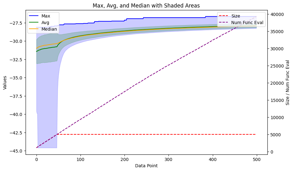
This process typically takes a few minutes to run. After completion, the ga_results variable contains information about the progression of the fitness of the population. We will utilize the same plot function as in the previous blog post to visualize the results.

plot_ga(ga_results.gen_info)

    <module 'matplotlib.pyplot' from '/home/esben/envs/molll/lib/python3.10/site-packages/matplotlib/pyplot.py'>

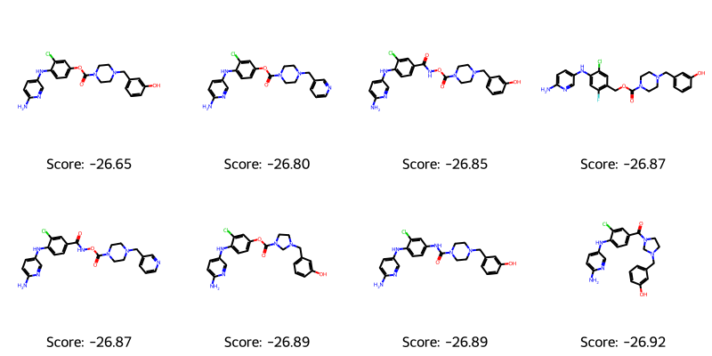
It’s also important to visually inspect the molecules themselves. Therefore, we will plot the top scoring ones for examination

best_mols = get_top_ten_tuples(ga_results.population)
visualize_molecules_with_scores(best_mols)

The molecules appear to lack unusual motifs and are of a reasonable size. However, they all look somewhat similar (and perhaps a bit boring?). Ensuring diversity and avoiding mode collapse is yet another challenge to address in generative modeling. The score is a combination of the log-likelihood estimate and the QSAR score, hence the negative number. However, we can quickly validate the QSAR model’s predictions of the generated SMILES strings. The best_mols variable contains tuples with (score, SMILES), so we will need to unpack to a list of SMILES strings.

integrated_model.predict([t[1] for t in best_mols])

    array([8.74559059, 8.52318629, 9.03374578, 8.59815202, 8.81134148,
           8.45991112, 8.59489244, 8.36500286])

They fall within the higher end of the score distribution from the dataset (cf. previous blog-post), although they do not exceed the maximum score. More freedom to optimize the QSAR score can be obtained by lowering the weight or alternative using it as a filter to avoid molecules with the lowest log-likelihood estimates under a given threshold (i.e. combined score = qsar_score*(ll_scores < threshold)). However, the choice of approach is ultimately up to the reward engineer. Whether it’s considered a positive outcome that we stay within the applicability domain or viewed as a failure of the restrained optimization is open for discussion. Feel free to share your thoughts and insights in the comments section below.
Good luck with the molecular optimizations and generations!

Best regards,
Esben

 

References:

1. Bjerrum EJ. Data Driven Estimation of Molecular Log-Likelihood using Fingerprint Key Counting. ChemRxiv. 2024; doi:10.26434/chemrxiv-2024-hzddj