Generating Unusual Molecules with Genetic Algorithms
I’ve long been working with generative models, mostly centered around SMILES-based deep learning models. However, I’ve been wanting to try out genetic algorithms for some time. Using the evolutionary mechanics inspired by Darwin as a template for optimizing a population, algorithms based on these principles have shown promising results in various domains, including molecular generation and optimization. Numerous studies, such as those referenced in this blog post (see: https://arxiv.org/abs/2310.09267 and https://arxiv.org/abs/2206.12411), have demonstrated competitive outcomes.
In this blog post, I aim to recreate some weird molecules, as it has been shown that generative models can produce unusual results when overexploiting Quantitative Structure-Activity Relationship (QSAR) models (e.g. see: https://doi.org/10.1016/j.ddtec.2020.09.003). First, we will build a QSAR model of activity using Scikit-Mol [1] in conjunction with Scikit-learn. We’ll use a dataset released as part of the mentioned paper, which originates from a binding assay against Tyrosine-protein kinase JAK2.
First step is to download and load the dataset into a pandas dataframe. A quick little helper function to either load it or download it can come in handy.
import os
import pandas as pd
import urllib.parse
import urllib.request
def load_csv_from_url(url, filename=None):
    if filename is None:
        filename = os.path.basename(urllib.parse.urlsplit(url).path)
    if not os.path.isfile(filename):
        urllib.request.urlretrieve(url, filename)

    df = pd.read_csv(filename)
    return df
url = "https://raw.githubusercontent.com/ml-jku/mgenerators-failure-modes/master/assays/processed/CHEMBL3888429.csv"
df = load_csv_from_url(url)
df.head()
| smiles | value | label | |
|---|---|---|---|
| 0 | NC(=O)c1cn(nc1Nc2ccnc(F)c2)C3(CC#N)CCN(Cc4cccn… | 6.84 | 0 |
| 1 | CN(C1CCC(CC#N)(CC1)n2cc(C(=O)N)c(Nc3ccnc(F)c3)… | 6.98 | 0 |
| 2 | NC(=O)c1cn(nc1Nc2ccc(F)cc2)C3(CC#N)CCN(CC3)C(=… | 7.48 | 0 |
| 3 | NC(=O)c1cn(nc1Nc2ccnc(F)c2)C3(CC#N)CCN(CC3)C(=… | 8.05 | 1 |
| 4 | NC(=O)c1cn(nc1Nc2ccnc(F)c2)C3(CC#N)CCC(CC3)NCc… | 8.70 | 1 |
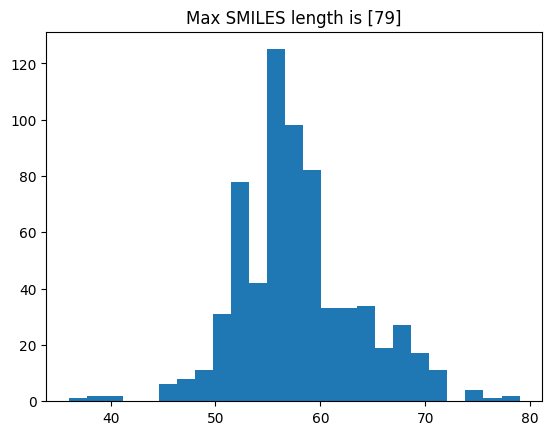
Good. The value to build the regression model from is in the “values” column, and it seems that high numbers are associated with being class 1, which should be active. Full details should be available in the paper mentioned before. Next, we will have a look at the properties of the dataset by examining distributions of the scores and SMILES string length, as we will need that info later on.
import matplotlib.pyplot as plt
length_smiles = df.smiles.apply(len)
_ = plt.hist(length_smiles, bins=25)
_ = plt.title(f"Max SMILES length is [{max(length_smiles)}]")
_ = plt.hist(df.value, bins=25)
_ = plt.title(f"Max value in y_train is [{max(df.value)}]")

I also always think it’s a good idea to look at the molecules (and that dataset contains some I would normally filter away), but for the sake of staying close to the paper, we’ll use the dataset as is and simply look at the top-valued molecules, which we can then use as a reference to gauge the later generated ones.
Turns out there is a NaN in the values column that we need to remove.
df = df[~df.value.isna()] #value contains some NaN's, must be filtered
from rdkit import Chem
from rdkit.Chem import Draw
from rdkit.Chem import AllChem
import numpy as np
#We feed in tuples of scores, smiles as this makes it easier for the output from the genetic algorithm further down....
def visualize_molecules_with_scores(molecule_data):
    mols = [Chem.MolFromSmiles(smiles) for _, smiles in molecule_data]
    img = Draw.MolsToGridImage(mols, molsPerRow=4, subImgSize=(200, 200), legends=[f'Score: {score:.2f}' for score, _ in molecule_data])
    return img
#Identify the top 8 and create the list of (scores, smiles)
top_indices = np.argsort(df.value)[::-1][:8]
top_molecules_and_scores = list(zip(df.value.values[top_indices],df.smiles.values[top_indices]))
visualize_molecules_with_scores(top_molecules_and_scores) # Pandas could probably give me the top 8 if I googled it
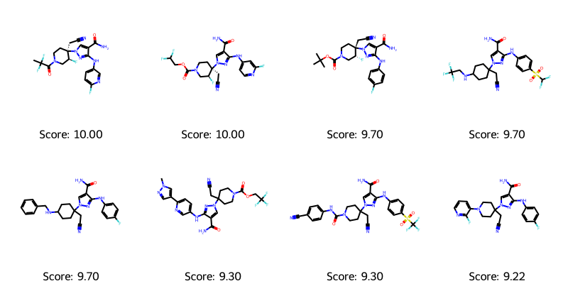
Now we have an idea of some of the chemical motifs that give a good score. Let’s go on and do some imports and build a simple Scikit-Learn model. First, some imports, splitting the dataset, and transforming the molecules into features. We use Scikit-Mol (https://pypi.org/project/scikit-mol/), which was introduced in another blog post, to handle our featurization. We keep it simple and standard with Morgan bit-fingerprints with a default radius (two).
from sklearn.model_selection import train_test_split
from sklearn.pipeline import Pipeline
from sklearn.linear_model import Ridge
from sklearn.model_selection import GridSearchCV
from scikit_mol.fingerprints import MorganFingerprintTransformer
from scikit_mol.conversions import SmilesToMolTransformer
X_train, X_test, y_train, y_test = train_test_split(df.smiles, df.value, test_size=0.2, random_state=42) #Good ol'e train_test_split
# Define the Feature Transformer
morgantrf = MorganFingerprintTransformer()
smilestrf = SmilesToMolTransformer()
feature_pipeline = Pipeline([
    ('smiles2mol', smilestrf),
    ('morgan', morgantrf)
])
X_train_transformed = feature_pipeline.transform(X_train)
X_test_transformed = feature_pipeline.transform(X_test)
print(f"X_train_transformed shape is {X_train_transformed.shape}")
X_train_transformed shape is (510, 2048)
With the features now in place, we build a simple Ridge Regression and tune the alpha parameter using GridSearchCV.
ridge_model = Ridge()
alpha_space = [0.1,10000]
param_grid = {'alpha': np.logspace(np.log10(alpha_space[0]), np.log10(alpha_space[1]), num=50)}
grid_search = GridSearchCV(estimator=ridge_model, param_grid=param_grid, scoring='neg_root_mean_squared_error', cv=3, return_train_score=True)
grid_search.fit(X_train_transformed, y_train) # CV is used to tune, NEVER the external test-set!!!
print(f"Best Alpha: {grid_search.best_params_['alpha']}")
print(f"Average NegRMSE on Training Set: {np.mean(grid_search.cv_results_['mean_train_score'])}")
print(f"Average NegRMSE on Cross-Validation Set: {np.mean(grid_search.cv_results_['mean_test_score'])}")
    Best Alpha: 10.985411419875584
    Average NegRMSE on Training Set: -0.5993705568456518
    Average NegRMSE on Cross-Validation Set: -0.7895764660492637
Let’s quickly test the scores, which for an sklearn Ridge regressor is the coefficient of determination R².
model = grid_search.best_estimator_
print("Train score:", model.score(X_train_transformed, y_train))
print("Test Score:", model.score(X_test_transformed, y_test))
    Train score: 0.6410330315855475
    Test Score: 0.3533566781607195
Not the best model I’ve ever made, but as we want to over-exploit it’s probably better to have a not too great model (E.g. see https://doi.org/10.1186/s13321-022-00601-y). We’ll quickly integrate the featurizer and transformer for easy integration in a few steps.
integrated_model = Pipeline((("Featurizer",feature_pipeline),("RidgeRegressor",model)))
integrated_model
Pipeline(steps=(('Featurizer',
                 Pipeline(steps=[('smiles2mol', SmilesToMolTransformer()),
                                 ('morgan', MorganFingerprintTransformer())])),
                ('RidgeRegressor', Ridge(alpha=10.985411419875584))))
Pipeline(steps=(('Featurizer',
                 Pipeline(steps=[('smiles2mol', SmilesToMolTransformer()),
                                 ('morgan', MorganFingerprintTransformer())])),
                ('RidgeRegressor', Ridge(alpha=10.985411419875584))))
Pipeline(steps=[('smiles2mol', SmilesToMolTransformer()),
                ('morgan', MorganFingerprintTransformer())])
SmilesToMolTransformer()
MorganFingerprintTransformer()
Ridge(alpha=10.985411419875584)
A quick test to see that it works….
integrated_model.predict(["c1ccccc1", "CO"])
array([5.64209907, 5.49391141])
With the model now in place, we can finally get to the fun part: using a genetic algorithm to generate some molecules with a good score! I’ve used the mol-ga project, a well-made package with an installer and tests. It has also been put on PyPI, so it’s very fast to install via pip. The genetic algorithm can be loaded and used with a few simple Python lines. Go ahead and pip install mol-ga if you haven’t already (mol-ga on PyPI: https://pypi.org/project/mol-ga/). Alternatively, visit the GitHub repository (mol-ga on GitHub: https://github.com/AustinT/mol_ga), clone, and install from there if you want to hack or experiment a bit with the code or simply want to understand better how it works.
There’s an example from the readme that I almost use exactly as shown here. I lowered the number of generations significantly as it very quickly does something that slows everything down. I also put the population size down so that it’s easier to follow the progress of the population even over a few generations.
import joblib
from rdkit import Chem
from mol_ga import mol_libraries, default_ga
start_smiles = mol_libraries.random_zinc(1000)
with joblib.Parallel(n_jobs=-1) as parallel:
        ga_results = default_ga(
            starting_population_smiles=start_smiles,
            scoring_function=integrated_model.predict, #How nice it is that the model can read lists of SMILES :-)
            max_generations=7,
            offspring_size=100,
            parallel=parallel,
            population_size=200, #Should efficiently make it more batch looking, but probably also more prone to mode-collapse
        )
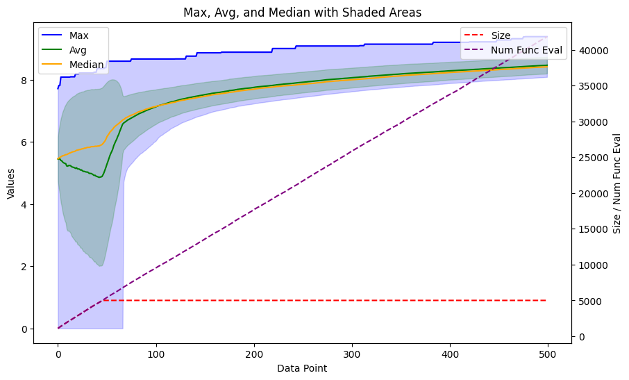
The ga_results is an object that contains the final population and the progress of the population in statistical metrics. I made a function to plot the progress using matplotlib.
def plot_ga(data):
    max_values = [entry['max'] for entry in data]
    avg_values = [entry['avg'] for entry in data]
    median_values = [entry['median'] for entry in data]
    min_values = [entry['min'] for entry in data]
    std_values = [entry['std'] for entry in data]
    size_values = [entry['size'] for entry in data]
    num_func_eval_values = [entry['num_func_eval'] for entry in data]
    fig, ax1 = plt.subplots(figsize=(10, 6))
    ax1.plot(max_values, label='Max', color='blue')
    ax1.plot(avg_values, label='Avg', color='green')
    ax1.plot(median_values, label='Median', color='orange')
    ax1.fill_between(range(len(data)), min_values, max_values, color='blue', alpha=0.2)
    ax1.fill_between(range(len(data)), np.subtract(avg_values, std_values), np.add(avg_values, std_values), color='green', alpha=0.2)
    ax1.set_xlabel('Data Point')
    ax1.set_ylabel('Values')
    ax1.set_title('Max, Avg, and Median with Shaded Areas')
    ax2 = ax1.twinx()
    ax2.plot(size_values, label='Size', linestyle='--', color='red')
    ax2.plot(num_func_eval_values, label='Num Func Eval', linestyle='--', color='purple')
    ax2.set_ylabel('Size / Num Func Eval')
    ax1.legend(loc='upper left')
    ax2.legend(loc='upper right')
    return plt
plot_ga(ga_results.gen_info)
<module 'matplotlib.pyplot' from '/home/esben/python_envs/vscode/lib/python3.10/site-packages/matplotlib/pyplot.py'>
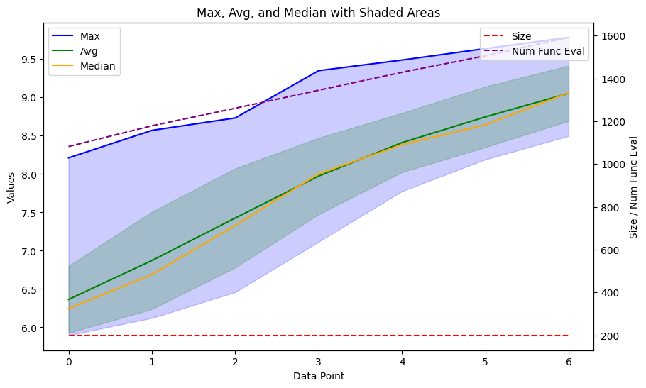
We see a nice progress in the scores, increasing very fast over just a couple of generations. Now, let’s look at how the molecules look. The plot_function from before works nicely for the .population data, which consists of tuples of scores and SMILES. First, let’s get the top 8.
def get_top_ten_tuples(input_list, k=8):
    numbers = np.array([float(item[0]) for item in input_list])
    top_indices = np.argsort(numbers)[::-1][:k]
    top_ten_tuples = [input_list[i] for i in top_indices]
    return top_ten_tuples
best_mols = get_top_ten_tuples(ga_results.population)
visualize_molecules_with_scores(best_mols)
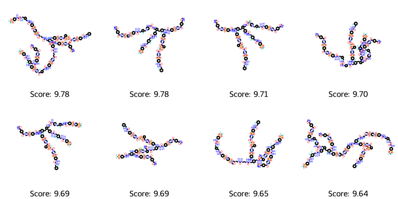
Oh, they seem really big! It appears we are definitely outside the applicability domain of the model. I tried various other settings of the featurizer for the model, and it seems to be a consistent thing that it drives towards bigger molecules. Perhaps it’s easier to keep and combine high-scoring features when crossing most of the parent molecules over? It also explains why everything slowed to a crawl with 100 generations. Anyway, we may want to impose restrictions on the size of the molecules.
We could probably write a SMILES to molecular weight (MW) transformer and include it in the integrated model via the FeatureUnion from scikit-learn, but this small wrapper function also works. To keep things simple, I use the SMILES string length rather than an atom count or MW, which may make more chemical sense. I’m also not sure if the SMILES strings are generated with the same settings (e.g., kekulized SMILES are longer than the corresponding aromatic SMILES), but let’s see if we can restrict the size and still generate weird-looking molecules.
def length_restricted_scoring(smiles_list):
smiles_lengths = np.array([len(smiles) for smiles in smiles_list])
scores = integrated_model.predict(smiles_list)
final_scores = (smiles_lengths &lt; 80) * scores #Largest from dataset was 74
return list(final_scores)
with joblib.Parallel(n_jobs=-1) as parallel:
    ga_results = default_ga(
        starting_population_smiles=start_smiles,
        scoring_function=length_restricted_scoring,
        max_generations=500,
        offspring_size=100,
        parallel=parallel,
        population_size=5000,
    )
plot_ga(ga_results.gen_info)
<module 'matplotlib.pyplot' from '/home/esben/python_envs/vscode/lib/python3.10/site-packages/matplotlib/pyplot.py'>
best_mols = get_top_ten_tuples(ga_results.population)
visualize_molecules_with_scores(best_mols)
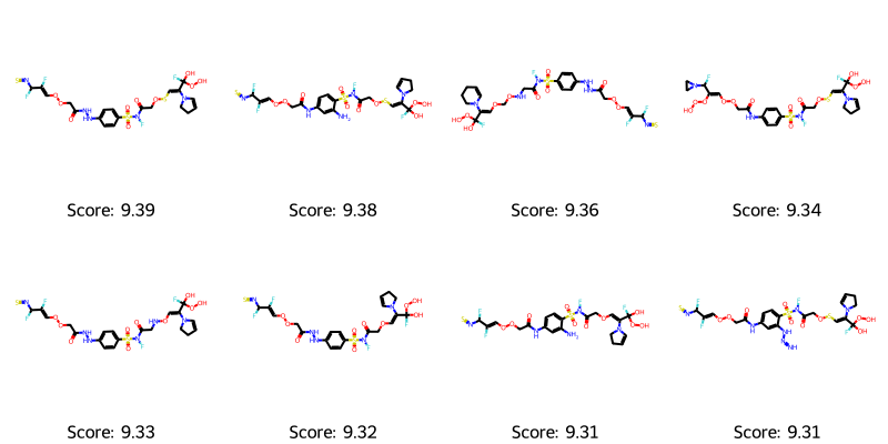
It definitely helped to restrict the SMILES length, addressing the size problem. However, we still often see unusual motifs in the molecules, such as R-NSNSNS, R-OSSH, NN, OF, OOO, C(F)(O)OO which are examples I’ve observed in different runs. I’m not sure I would be proud of those motifs if I were trying to generate drug-like molecules. If you redo this, please comment below with the weirdest motifs or molecules you find.
Running long enough, we also get molecules with a score higher than the top for the training set. Comparing it to the actives from the training set (see above), I think we can often recognize motifs and sub-patterns that are similar to the ones found in the top-known ligands.
To achieve good results, it seems like we would have to carefully build up the scoring function with filters against unusual functional groups, restrictions on molecular weight, and couple it with SA-score and QED scores, etc. I hope this illustrates how a Genetic algorithm can quickly optimize molecules towards a given scoring function, but that we also need to watch closely what kind of molecules we get generated.
Best of luck with your molecule generation and optimization
References
[1] Bjerrum, Esben Jannik, Rafał Adam Bachorz, Adrien Bitton, Oh-hyeon Choung, Ya Chen, Carmen Esposito, Son Viet Ha, and Andreas Poehlmann. “Scikit-Mol Brings Cheminformatics to Scikit-Learn.” ChemRxiv, December 6, 2023. https://doi.org/10.26434/chemrxiv-2023-fzqwd.
Hi Esben
I liked your post a lot. what about PAINS to filter?
Thanks. Pains filters could maybe filter some of these out, but I don’t think that is the aim of the PAINS filters.
Cool stuff. Isn’t the issue of genetic generation as old as the any other genetic algorithm, i.e. it will create weird motifs unless they are is a blacklist?
And as for any current NN approach, the system don’t really “know chemistry” as much as we want them to learn.
My favorite motif after this excercise in my case btw was -NH-NH-N=O and NH-N(-CL)-NH ….
😀
At least hybridization is correct…
Yes, indeed, it seems to be a culprit with GA methods. Glad you made it work and got some novel molecules 😉
Take a look at the github repo molskillscore. It was trained by the eye of medchemists and could provide a means of prioritising molecules that would ‘look better’ for development in an intelligently biased fashion.
Also rdkit has a simple function to calculate weights but not clear how to add that prospectively.
Thanks for the interest and for commenting. If you try out using mollskillscore to guide generation, please comment with your experiences
Pingback: Generating Unusual Molecules with Genetic Algorithms Part 2: Leveraging MolLL for Enhanced Generation | Cheminformania