Tune your deep tox neural network with free tools

Esben Jannik Bjerrum/ February 7, 2017/ Blog, Machine Learning, Neural Network/ 3 comments

In another blog post I demonstrated how to build a deep neural network with Keras in Python to model some toxicity dataset from the Tox21 challenge. The network was however not systematically optimized, but merely put together with a few manually selected hyper parameters. Hyper parameters are understood as the parameters which are not tuned by the data through training, such as number of hidden layers, number of neurons, dropout rate, l2 regularization penalty and so forth. For neural networks there exists a lot of choices to be made and thus a lot of hyper parameters, which can make it a complicated affair.
Luckily there are a lot of interesting machine learning tools out there, and specifically Gaussian Process Optimization or Bayesian Optimization has been widely employed to find a good set of hyper parameters for neural networks. We can thus tune our machine learning algorithm by using another machine learning algorithm, and I’ll show below how this is done with the python package GPyOpt.
The method works by exploring points of an unknown function and then fit a model to these, here a Gaussian processes model. Instead of just trying to minimizing the function, the Gaussian process optimization uses a combination of the expected fitness with the uncertainty of the model. The next point to explore is thus not chosen directly as the predicted minimum of the function, but also from an area where the model has a high uncertainty. This behavior of the optimization is controlled by an acquisition function, which ironically enough often has its own hyper parameter that balances exploration (testing unknown areas) with exploitation (testing places with expected low values of the loss function). The documentation for GPyOpt have a nice step by step demonstration of the process.
In order to optimize the neural network, the construction of the network is embedded in a function that takes the tested hyper parameters, constructs the network and returns the loss function. All the data loading, standardization and calculation of molecular fingerprints were done as in the previous post.

def deeptoxnn(l1 = 0.0, l2= 0.0, dropout = 0.0, dropout_in=0.0, hiddendim = 4, hiddenlayers = 3, lr = 0.001, nb_epoch=50, returnmodel=False):
	#Build neural network
	model = Sequential()
	model.add(Dropout(dropout_in, input_shape=(X_train.shape[1],)))
	for i in range(hiddenlayers):
		wr = WeightRegularizer(l2 = l2, l1 = l1)
		model.add(Dense(output_dim=hiddendim, activation="relu", W_regularizer=wr))
		model.add(Dropout(dropout))
	wr = WeightRegularizer(l2 = l2, l1 = l1)
	model.add(Dense(y_train.shape[1], activation='sigmoid',W_regularizer=wr))
	##Compile model and make it ready for optimization
	model.compile(loss='binary_crossentropy', optimizer = SGD(lr=lr, momentum=0.9, nesterov=True), metrics=['binary_crossentropy'])
	#Reduce lr callback
	reduce_lr = ReduceLROnPlateau(monitor='loss', factor=0.5,patience=10, min_lr=0.000001, verbose=returnmodel)
	#Save best model (Early stopping)
	modelcp = ModelCheckpoint("tempmodel.h5", monitor='val_loss', verbose=returnmodel, save_best_only=True)
	#Training
	history = model.fit(X_train, y_train, nb_epoch=nb_epoch, batch_size=1000, validation_data=(X_val,y_val), callbacks=[reduce_lr, modelcp], verbose=returnmodel)
	loss = history.history["val_loss"][-1]
	if returnmodel:
		return loss,model, history
	else:
		return loss

The GPyOpt expects the fitness function to take a 2D numpy array with multiple sets of hyper parameters and return multiple results from the function. As the neural network modeling is only running in serial due to restrictions of my hardware, a simple wrapper function has to be written to feed the hyper parameters to the neural network function we just defined.

def fit_nn_val(x):
	x = np.atleast_2d(x)# Must take a 2 D array with parms
	fs = np.zeros((x.shape[0],1)) #prepare return array with similar return dimension
	for i in range(x.shape[0]):
		val_loss = deeptoxnn(l2=float(x[i,0]),dropout=float(x[i,1]), dropout_in=float(x[i,2]),lr=float(x[i,3]), hiddendim=int(x[i,4]),hiddenlayers=int(x[i,5]))
		fs[i] = np.log(val_loss)
	print val_loss, fs
	return fs

We need to define a search space for the optimization process, which for GPyOpt is done with a list of dictionaries. Here it is also defined if a value is discrete like the number of neurons or the number of hidden layers.

#Discrete Variable must be at the end
mixed_domain =[ {'name': 'l2', 'type': 'continuous', 'domain': (0.0,0.07)},
		{'name': 'dropout', 'type': 'continuous', 'domain': (0.0,0.7)},
		{'name': 'dropout_in', 'type': 'continuous', 'domain': (0.0,0.5)},
		{'name': 'lr', 'type': 'continuous', 'domain': (0.0001,0.1)},
               {'name': 'hiddendim', 'type': 'discrete', 'domain': [2**x for x in range(2,7)]},
               {'name': 'hiddenlayers', 'type': 'discrete', 'domain': range(1,3)}]

For the actual optimization, the GP_MCMC model with the EI_MCMC acquisition seems to work fine. Its a modified optimization process which according to this paper should work more efficient.  The model initially explores 50 random points for the first fit of the model. This number is much higher than the default (5), but we are exploring a complex and noisy 8 dimensional hyper parameter space. This leads to the Gaussian Processes fit using the CPU to actually take more time than building and optimizing the neural network with the GPU. Additionally, Sampling many random points initially also helps to minimize the risk of getting trapped in a local minima. After the initial sampling, the model explores an additional 100 points at maximum.

myBopt = BayesianOptimization(f=fit_nn_val,                   # function to optimize
                              domain=mixed_domain,        # box-constrains of the problem
                              initial_design_numdata = 50,# number data initial design
			      model_type="GP_MCMC",
                              acquisition_type='EI_MCMC', #EI
			      evaluator_type="predictive",  # Expected Improvement
			      batch_size = 1,
                              num_cores = 4,
                              exact_feval = False)         # May not always give exact results
myBopt.run_optimization(max_iter = 100)
x_best = myBopt.x_opt #myBopt.X[np.argmin(myBopt.Y)]
print x_best
myBopt.plot_convergence()

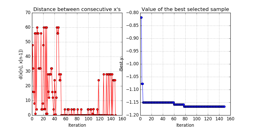
Looking at the convergence plots we see to the right that it found the best solution after approximately 75 tries, after which the optimization explored a further 75 points.

It actually also found a very good solution in the random sampling period. So what hyper parameters worked the best?

[  6.81787644e-03   1.76266330e-02   9.99502028e-02   8.24763920e-02
   8.00000000e+00   1.00000000e+00]

So it seems like the optimally found parameters have only 1 layer and 8 neurons.
But hey, wait! If there’s only one layer, can we still call the network “deep”?
A: No, with neural networks, we count the layers one – two – deep.
🙁
A: But its still a neural network. And now its optimized!
😐
A: And you still get to use cool regularization techniques like dropout.
🙂
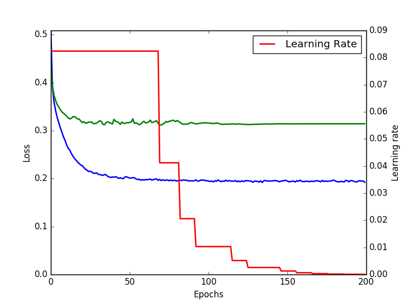
The wrapper code is used to build the model, but instead of 50 epochs we try and train it for 200. The training shows that the model is stable and do not over fit due to prolonged training.

val_loss, model, history = deeptoxnn(l2=6.81e-3, dropout=1.76e-2, dropout_in=9.99e-2,lr=8.24e-02, nb_epoch = 200, hiddendim=8,hiddenlayers=1, returnmodel=True)
#Reporting
plot_history(history)

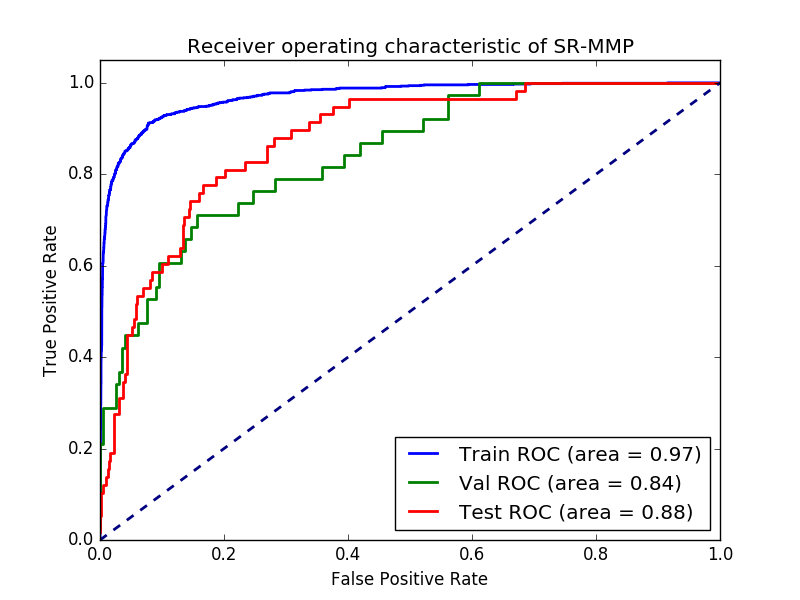
Like in the last post we use a receiver operator curve plot and calculate the area under the curve to gauge the model.

show_auc(model)

This looks much better than last time, and has a much higher AUC for the external test set (0.88 vs. 0.77 last time). Deep is not always better. This is really one of the good things doing some more automatic optimization. That one gets out in corner cases, which for one or the other reason was not considered.
Cheers
Esben