Master your molecule generator: Seq2seq RNN models with SMILES in Keras
UPDATE: Be sure to check out the follow-up to this post if you want to improve the model: Learn how to improve SMILES based molecular autoencoders with heteroencoders
I’ve previously written about molecular generators based on long short-term memory recurrent neural networks (LSTM-RNNs). The networks learn rules about how SMILES strings of molecules are formatted and are then able to create novel SMILES following the same rules by iterating through the characters. The results are “creative” computers that can draw correct molecules.
An interesting aspect is that the distribution of molecular properties are the same for the training dataset and the later samples https://arxiv.org/abs/1705.04612. “You get what you train for” could sound like a commercial for a fitness center but equally apply here.
However it takes a few thousand molecules to train one of these character based generators without over-fitting and getting the chemical rules underlying the SMILES generation correct. Pre-training on larger datasets work to some degree, but the molecules anyway end up looking strange with unlikely anti-aromatic rings.
Another approach is to make an autoencoder. The basic idea is to code the input (here SMILES strings) string to a latent space and then recreate the original input from this space. After training, the autoencoder can be split into an encoder and a decoder. The decoder can be used to sample the area around a molecule of interest (Lead-compound?) and generate similar, but not equal, molecules.
I have also written about my experiences using keras-molecules to map molecules to latent space with subsequent visualization. This code uses a convolutional encoder and a GRU based decoder.
However, it should also be possible to use an RNN based encoder, which was done by Zheng Xu and Co-workers. Their code doesn’t seem to be readily available, but read on below and see how it can be implemented with Keras.
# General Imports
import os
import pandas as pd
import numpy as np
from rdkit import Chem
from rdkit.Chem import Draw, Descriptors
from matplotlib import pyplot as plt
%matplotlib inline
There is of course a need for some SMILES strings to train and test on. To keep things a bit simple (and training shorter) for this blog post, the file with SMILES containing 8 atoms from the GDB-11 dataset will be used. It contains all molecules possible to generate with a subset of atoms and bond types. The dataset can be downloaded here: http://gdb.unibe.ch/downloads/. A random split into train- and test-set is done immediately before further processing.
smifile = "gdb11_size08.smi"
data = pd.read_csv(smifile, delimiter = "\t", names = ["smiles","No","Int"])
from sklearn.cross_validation import train_test_split
smiles_train, smiles_test = train_test_split(data["smiles"], random_state=42)
print smiles_train.shape
print smiles_test.shape
    (50029,)
    (16677,)
The SMILES must be vectorized to one-hot encoded arrays. To do this a character set is built from all characters found in the SMILES string (both train and test). Also, some start and stop characters are added, which will be used to initiate the decoder and to signal when SMILES generation has stopped. The stop character also work as padding to get the same length of all vectors, so that the network can be trained in batch mode. The character set is used to define two dictionaries to translate back and forth between index and character. The maximum length of the SMILES strings is needed as the RNN’s will be trained in batch mode, and is set to the maximum encountered + some extra.
charset = set("".join(list(data.smiles))+"!E")
char_to_int = dict((c,i) for i,c in enumerate(charset))
int_to_char = dict((i,c) for i,c in enumerate(charset))
embed = max([len(smile) for smile in data.smiles]) + 5
print str(charset)
print(len(charset), embed)
    set(['!', '#', ')', '(', '+', '-', '1', '3', '2', '4', '=', 'C', 'E', 'F', 'H', 'O', 'N', '[', ']', 'c', 'o', 'n'])
    (22, 28)
Afterwards the character set and dictionaries are used to set the necessary bits in the Numpy arrays. The result will be a “piano-roll” of each molecules SMILES string. The X data starts with !, but the output Y is offset by one character, and starts with the first character of the actual SMILES.
def vectorize(smiles):
        one_hot =  np.zeros((smiles.shape[0], embed , len(charset)),dtype=np.int8)
        for i,smile in enumerate(smiles):
            #encode the startchar
            one_hot[i,0,char_to_int["!"]] = 1
            #encode the rest of the chars
            for j,c in enumerate(smile):
                one_hot[i,j+1,char_to_int[[c]]] = 1
            #Encode endchar
            one_hot[i,len(smile)+1:,char_to_int["E"]] = 1
        #Return two, one for input and the other for output
        return one_hot[:,0:-1,:], one_hot[:,1:,:]
X_train, Y_train = vectorize(smiles_train.values)
X_test,Y_test = vectorize(smiles_test.values)
print smiles_train.iloc[0]
plt.matshow(X_train[0].T)
#print X_train.shape
N#CC#CC1COC1
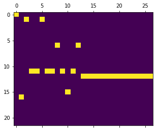
The int_to_char dictionary can be used to go from vectorized form back to a readable string, here with a joined list comprehension.
"".join([int_to_char[idx] for idx in np.argmax(X_train[0,:,:], axis=1)])
'!N#CC#CC1COC1EEEEEEEEEEEEEE'
With the vectorized data ready, it time to build the autoencoder. First some Keras objects will be imported and the dimensions for the input and output calculated from the vectorized data. Additionally the number of LSTM cell to use for the decoder and encoder is specified and the latent dimension is specified.
#Import Keras objects
from keras.models import Model
from keras.layers import Input
from keras.layers import LSTM
from keras.layers import Dense
from keras.layers import Concatenate
from keras import regularizers
input_shape = X_train.shape[1:]
output_dim = Y_train.shape[-1]
latent_dim = 64
lstm_dim = 64
Using TensorFlow backend.
Long Short-Term Memory Cells (LSTM)
It may sound like an oxymoron, but long short-term memory cells are special kinds of neural network units that are designed to keep an internal state for longer iterations through a recurrent neural network. They have been designed with input, output and forget gates, that control what to do with the cells internal state C. The state H is passed as a copy between the recurrent iterations and helps determine what should be done with the internal state C in the next iteration. The gating mechanisms ensures that the network can easily retain an internal state by closing off the input and forget gates until a new condition or input opens them. They work as drop-in replacements for standard recurrent units and usually increase the performance of the RNN with regard to recognizing long term interactions. Luckily they are already implemented in Keras. An also popular, simplified version is the gated recurrent unit (GRU) that is also available in Keras.
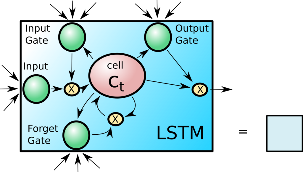
The model is overall kept rather simple. A single layer of 64 LSTM cells is used to read the input SMILES string. The outputs from the layer is ignored, but the final internal C and H state is concatenated and recombined into a the bottleneck layer “neck”. This comprises the encoder.
The functional API of Keras is used and this will make it easier to rebuilt the various layers into encoder and decoder models later.
unroll = False
encoder_inputs = Input(shape=input_shape)
encoder = LSTM(lstm_dim, return_state=True,
                unroll=unroll)
encoder_outputs, state_h, state_c = encoder(encoder_inputs)
states = Concatenate(axis=-1)([state_h, state_c])
neck = Dense(latent_dim, activation="relu")
neck_outputs = neck(states)
The neck_output tensor is then put through two different Dense layers to decode the states that should be set on the decoder LSTM layer. This recombination of the internal states from the encoder to decoder, makes it possible to use a different size latent space than encoded by the LSTM layers in themselves. The LSTM layer then receives the input once again, and is put to the task of predicting the next character in the sequence. So from the latent representation of the molecule and the character “!”, it should output what the next character is, representing the first atom, e.g. “C”, “N” etc. This is why the Y vectors are offset from the X vectors with the “!”character. This way of training is called teacher enforcing in contrast to the approach where the output of one recurrence step is used as input to the next. Even though the network may make a mistake in the start of the sequence, it will not affect the training of the later parts of the sequence. This trains the decoder much more efficiently, than just feeding it the internal states and then see if it can construct the whole sequence. The LSTM cells output at each step is put into a Dense network with each neurons task to predict the correct character.
The final model for training is then built from the input-layer objects and the output layer.
decode_h = Dense(lstm_dim, activation="relu")
decode_c = Dense(lstm_dim, activation="relu")
state_h_decoded =  decode_h(neck_outputs)
state_c_decoded =  decode_c(neck_outputs)
encoder_states = [state_h_decoded, state_c_decoded]
decoder_inputs = Input(shape=input_shape)
decoder_lstm = LSTM(lstm_dim,
                    return_sequences=True,
                    unroll=unroll
                   )
decoder_outputs = decoder_lstm(decoder_inputs, initial_state=encoder_states)
decoder_dense = Dense(output_dim, activation='softmax')
decoder_outputs = decoder_dense(decoder_outputs)
#Define the model, that inputs the training vector for two places, and predicts one character ahead of the input
model = Model([encoder_inputs, decoder_inputs], decoder_outputs)
print model.summary()
    __________________________________________________________________________________________________
    Layer (type)                    Output Shape         Param #     Connected to
    ==================================================================================================
    input_9 (InputLayer)            (None, 27, 22)       0
    __________________________________________________________________________________________________
    lstm_9 (LSTM)                   [(None, 64), (None,  22272       input_9[0][0]
    __________________________________________________________________________________________________
    concatenate_5 (Concatenate)     (None, 128)          0           lstm_9[0][1]
                                                                     lstm_9[0][2]
    __________________________________________________________________________________________________
    dense_15 (Dense)                (None, 64)           8256        concatenate_5[0][0]
    __________________________________________________________________________________________________
    input_10 (InputLayer)           (None, 27, 22)       0
    __________________________________________________________________________________________________
    dense_16 (Dense)                (None, 64)           4160        dense_15[0][0]
    __________________________________________________________________________________________________
    dense_17 (Dense)                (None, 64)           4160        dense_15[0][0]
    __________________________________________________________________________________________________
    lstm_10 (LSTM)                  (None, 27, 64)       22272       input_10[0][0]
                                                                     dense_16[0][0]
                                                                     dense_17[0][0]
    __________________________________________________________________________________________________
    dense_18 (Dense)                (None, 27, 22)       1430        lstm_10[0][0]
    ==================================================================================================
    Total params: 62,550
    Trainable params: 62,550
    Non-trainable params: 0
    __________________________________________________________________________________________________
    None
After preparing some Keras callbacks to record the history and reduce the learning rate once a training plateau is reached, the model is compiled with optimizer and loss function and the training can begin. Note how the X_train is fed two times to the model, to give the input at two different places in the model.
from keras.callbacks import History, ReduceLROnPlateau
h = History()
rlr = ReduceLROnPlateau(monitor='val_loss', factor=0.5,patience=10, min_lr=0.000001, verbose=1, epsilon=1e-5)
from keras.optimizers import RMSprop, Adam
opt=Adam(lr=0.005) #Default 0.001
model.compile(optimizer=opt, loss='categorical_crossentropy')
model.fit([X_train,X_train],Y_train,
                    epochs=200,
                    batch_size=256,
                    shuffle=True,
                    callbacks=[h, rlr],
                    validation_data=[[X_test,X_test],Y_test ])
    Train on 50029 samples, validate on 16677 samples
    Epoch 1/200
    50029/50029 [==============================] - 21s 417us/step - loss: 0.9442 - val_loss: 0.6275
.......
    Epoch 199/200
    50029/50029 [==============================] - 18s 363us/step - loss: 3.2088e-05 - val_loss: 2.5274e-04
    Epoch 200/200
    50029/50029 [==============================] - 18s 368us/step - loss: 3.1181e-05 - val_loss: 2.5532e-04
import pickle
pickle.dump(h.history, file("Blog_history.pickle","w"))
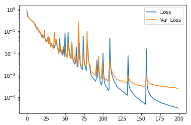
The training process can be plotted using the data recorded in the history object. There are some spikes in the loss and validation loss, but in the end the loss and validation loss levels more or less out. Note the Logarithmic scale make the growing difference between the loss and validation loss appear larger than it really is.
plt.plot(h.history["loss"], label="Loss")
plt.plot(h.history["val_loss"], label="Val_Loss")
plt.yscale("log")
plt.legend()
A quick test directly on the model, before we reassemble the trained parts into new models show that there is a good reconstruction accuracy also on the test set. The code below outputs nothing so the 100 tested SMILES from the test set is perfectly reconstructed.
for i in range(100):
    v = model.predict([X_test[i:i+1], X_test[i:i+1]]) #Can't be done as output not necessarely 1
    idxs = np.argmax(v, axis=2)
    pred=  "".join([int_to_char[h] for h in idxs[0]])[:-1]
    idxs2 = np.argmax(X_test[i:i+1], axis=2)
    true =  "".join([int_to_char[k] for k in idxs2[0]])[1:]
    if true != pred:
        print true, pred
Now the parts of the trained autoencoder will be used to build the various encoder and decoder models. Building a new model from the input layer to an output layer inside another model is very simple. The input layer defined when the model was built it reused and the neck_output reused as the output. This model will take a vectorized smile and encode it to the latent space.
smiles_to_latent_model = Model(encoder_inputs, neck_outputs)
smiles_to_latent_model.save("Blog_simple_smi2lat.h5")
The next model that will be needed is a model that can decode the latent space into the states that need to be set at the decoder LSTM cells. A new input matching the latent space is defined, but the layers from before can be reused to get the h and c states. That way the weights are inherited from the trained model.
latent_input = Input(shape=(latent_dim,))
#reuse_layers
state_h_decoded_2 =  decode_h(latent_input)
state_c_decoded_2 =  decode_c(latent_input)
latent_to_states_model = Model(latent_input, [state_h_decoded_2, state_c_decoded_2])
latent_to_states_model.save("Blog_simple_lat2state.h5")
The decoder model needs a bit more work. It was trained in batch mode, but it will be used in stateful mode predicting one character at a time. So the layers are defined precisely as before, except with a new batch_shape and the LSTM layer set to stateful.
#Last one is special, we need to change it to stateful, and change the input shape
inf_decoder_inputs = Input(batch_shape=(1, 1, input_shape[1]))
inf_decoder_lstm = LSTM(lstm_dim,
                    return_sequences=True,
                    unroll=unroll,
                    stateful=True
                   )
inf_decoder_outputs = inf_decoder_lstm(inf_decoder_inputs)
inf_decoder_dense = Dense(output_dim, activation='softmax')
inf_decoder_outputs = inf_decoder_dense(inf_decoder_outputs)
sample_model = Model(inf_decoder_inputs, inf_decoder_outputs)
After defining the decoder model, the corresponding weights from the trained autoencoder model are transfered.
#Transfer Weights
for i in range(1,3):
    sample_model.layers[i].set_weights(model.layers[i+6].get_weights())
sample_model.save("Blog_simple_samplemodel.h5")
sample_model.summary()
    _________________________________________________________________
    Layer (type)                 Output Shape              Param #
    =================================================================
    input_13 (InputLayer)        (1, 1, 22)                0
    _________________________________________________________________
    lstm_11 (LSTM)               (1, 1, 64)                22272
    _________________________________________________________________
    dense_19 (Dense)             (1, 1, 22)                1430
    =================================================================
    Total params: 23,702
    Trainable params: 23,702
    Non-trainable params: 0
    _________________________________________________________________
Using the latent space as a fingerprint
The smiles to latent model can be used to encode the SMILES into the fingerprint like latent space
x_latent = smiles_to_latent_model.predict(X_test)
A useful feature of a fingerprint is if similar molecules produces similar fingerprints. To see if similar molecules produce similar vectors in the latent space, a simple search for similar molecules can be performed. Here the absolute difference between the latent vectors is used as a metric of similarity. This test do not rule out that similar molecules can get latent vectors that are dissimilar, but is a quick test of the immediate neighborhood.
molno = 5
latent_mol = smiles_to_latent_model.predict(X_test[molno:molno+1])
sorti = np.argsort(np.sum(np.abs(x_latent - latent_mol), axis=1))
print sorti[0:10]
print smiles_test.iloc[sorti[0:8]]
Draw.MolsToImage(smiles_test.iloc[sorti[0:8]].apply(Chem.MolFromSmiles))
    [    5  1243 15472   744 15039 14589  2449  3991  5251 16502]
    45051    COCc1cocn1
    45007    COCc1ccoc1
    45061    COCc1conn1
    45025    CCOc1cnoc1
    45069    COCc1ncon1
    44719    COCc1ccno1
    45063    CCOc1conn1
    44727    COCc1cnno1
    Name: smiles, dtype: object

The first one is the query molecule. They do look similar, but maybe because the SMILES strings are very similar, rather than following our understanding of molecular similarity. Lets see what is the most different molecules in the latent spaces.
Draw.MolsToImage(smiles_test.iloc[sorti[-8:]].apply(Chem.MolFromSmiles))

Chemical properties in the latent space
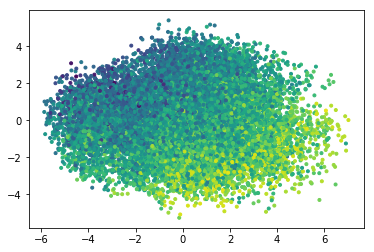
As a proxy for chemical properties, lets see how the calculated LogP and MR maps to a PCA reduction of the latent space
logp = smiles_test.apply(Chem.MolFromSmiles).apply(Descriptors.MolLogP)
from sklearn.decomposition import PCA
pca = PCA(n_components = 2)
red = pca.fit_transform(x_latent)
plt.figure()
plt.scatter(red[:,0], red[:,1],marker='.', c= logp)
print(pca.explained_variance_ratio_, np.sum(pca.explained_variance_ratio_))
(array([ 0.24815299, 0.15272172], dtype=float32), 0.4008747)
molwt = smiles_test.apply(Chem.MolFromSmiles).apply(Descriptors.MolMR)
plt.figure()
plt.scatter(red[:,0], red[:,1],marker='.', c= molwt)
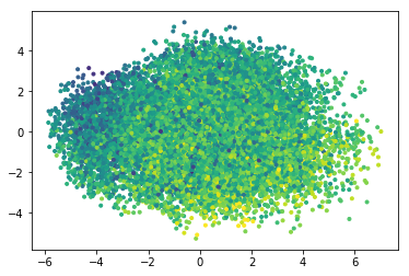
There seem to be some distribution of the predicted molecular properties.
Modeling properties from the latent space
It could also be interesting to see if the fingerprints work good as a basis for QSAR models. As a proxy for the target value of QSAR modelling, a model of the predicted LogP will be built. Building a model using a modeled property is only done for demonstration purposes.
#Model LogP?
x_train_latent = smiles_to_latent_model.predict(X_train)
logp_train = smiles_train.apply(Chem.MolFromSmiles).apply(Descriptors.MolLogP)
from keras.models import Sequential
logp_model = Sequential()
logp_model.add(Dense(128, input_shape=(latent_dim,), activation="relu"))
logp_model.add(Dense(128, activation="relu"))
logp_model.add(Dense(1))
logp_model.compile(optimizer="adam", loss="mse")
rlr = ReduceLROnPlateau(monitor='val_loss', factor=0.5,patience=10, min_lr=0.000001, verbose=1, epsilon=1e-5)
logp_model.fit(x_train_latent, logp_train, batch_size=128, epochs=400, callbacks = [rlr])
    Epoch 1/200
    50029/50029 [==============================] - 1s 25us/step - loss: 0.0236
.....
    Epoch 200/200
    50029/50029 [==============================] - 1s 23us/step - loss: 0.0187
logp_pred_train = logp_model.predict(x_train_latent)
logp_pred_test = logp_model.predict(x_latent)
plt.scatter(logp, logp_pred_test, label="Test")
plt.scatter(logp_train, logp_pred_train, label="Train")
plt.legend()
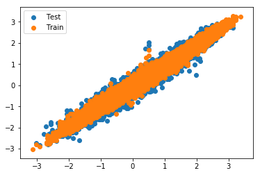
I would have expected even better fit when modeling a modeled property.
From latent space to SMILES
To sample the latent space, we need two steps. First compute the c and h states using the latent_to_states_model and then set the initial states of the decoder LSTM network. The LSTM network will be fed the input char vector and iteratively sample the next character until the end char “E” is encountered.
def latent_to_smiles(latent):
    #decode states and set Reset the LSTM cells with them
    states = latent_to_states_model.predict(latent)
    sample_model.layers[1].reset_states(states=[states[0],states[1]])
    #Prepare the input char
    startidx = char_to_int["!"]
    samplevec = np.zeros((1,1,22))
    samplevec[0,0,startidx] = 1
    smiles = ""
    #Loop and predict next char
    for i in range(28):
        o = sample_model.predict(samplevec)
        sampleidx = np.argmax(o)
        samplechar = int_to_char[sampleidx]
        if samplechar != "E":
            smiles = smiles + int_to_char[sampleidx]
            samplevec = np.zeros((1,1,22))
            samplevec[0,0,sampleidx] = 1
        else:
            break
    return smiles
smiles = latent_to_smiles(x_latent[0:1])
print smiles
print smiles_test.iloc[0]
    NCCC1OC=NO1
    NCCC1OC=NO1
It can be relevant to know how large a fraction of the SMILES are malformed when sampling the test set?
wrong = 0
for i in range(1000):
    smiles = latent_to_smiles(x_latent[i:i+1])
    mol = Chem.MolFromSmiles(smiles)
    if mol:
        pass
    else:
        print smiles
        wrong = wrong + 1
print "%0.1F percent wrongly formatted smiles"%(wrong/float(1000)*100)
    Cc1ccc(N)n[nH]1
    0.1 percent wrongly formatted smiles
This is actually quite good. Another interesting thing could be to see if the molecules can be “interpolated” in the latent space.
#Interpolation test in latent_space
i = 0
j= 2
latent1 = x_latent[j:j+1]
latent0 = x_latent[i:i+1]
mols1 = []
ratios = np.linspace(0,1,25)
for r in ratios:
    #print r
    rlatent = (1.0-r)*latent0 + r*latent1
    smiles  = latent_to_smiles(rlatent)
    mol = Chem.MolFromSmiles(smiles)
    if mol:
        mols1.append(mol)
    else:
        print smiles
Draw.MolsToGridImage(mols1, molsPerRow=5)
    NCCC1=ONCC1
    CC1=NCCCON1=C
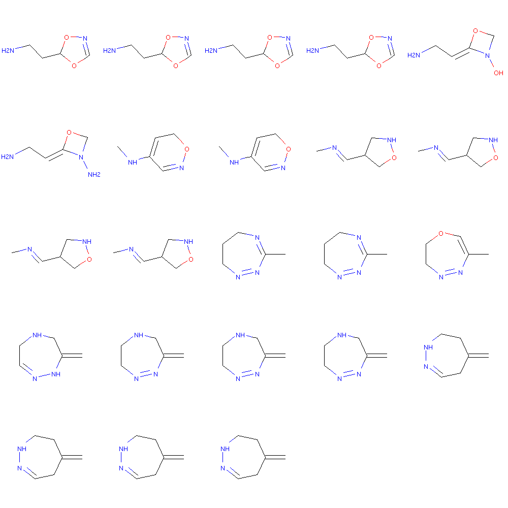
The mis sampling seem to be higher as two out of 25 molecules could not be parsed. The interpolation also shows how the same molecule is generated for slightly different areas of the latent space. This maybe reflects that the molecules are discrete and the latent space continuous, with a higher chance of failing when we are at the border between two molecules.
Another interesting property to examine is if novel molecules more or less similar to a lead molecule can be by adding a bit of randomness to an existing latent vector.
#Sample around the latent wector
latent = x_latent[0:1]
scale = 0.40
mols = []
for i in range(20):
    latent_r = latent + scale*(np.random.randn(latent.shape[1])) #TODO, try with
    smiles = latent_to_smiles(latent_r)
    mol = Chem.MolFromSmiles(smiles)
    if mol:
        mols.append(mol)
    else:
        print smiles
Draw.MolsToGridImage(mols, molsPerRow=5)
    NCCO1C=CC1O
    CONC(CCN1CO1
    NCC#CCCN1N
    NCCC=NO1CN1
    NCC1CO=CN1O
    NCCC1O(C)OO
    CNN1C(CFC1=O1
    NCC=CCO1N1
    COC1CC=NN=C
    NCCO1CCON1
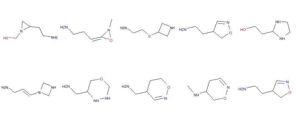
Here we really see a lot of wrong SMILES generated, but nevertheless see some molecules that may be more or less similar to the one used to encode the latent vector. (Compare to the first molecule in the interpolation above). Tuning the scaling can be a way to tune the creativity.
Summary
In this blog post it was shown how to make an LSTM based autoencoder of SMILES strings of molecules and efficiently train it with teacher enforcing. The latent space may reflect the structure of the SMILES but nevertheless seem useful for a variety of cheminformatics related tasks. The SMILES reconstruction accuracy seem to drop when bordering domains between molecules or adding random noise. Thus the latent space may not be completely continuous reflecting the discrete nature of the molecules. I’ve not mentioned AI in this blog-post as I’m not sure how to define intelligence in the first place, but I do find it fascinating how the chemical rules of SMILES strings can be picked up by the weights and computations done in the neural networks of the LSTM cells and later used to create novel SMILES strings.
Hello,
How can I save and load the model(s)?
The models are Keras models and are easily saved and loaded via the model.save(‘your_filename.h5’) and the load_model function from keras.models. You can read more in the Keras FAQ: https://keras.io/getting-started/faq/#how-can-i-save-a-keras-model.
But you will also need to save the char_to_int and int_to_char for correctly encoding and parsing the one-hot encoded characters when you want to use the models again. You can either use pickle and save to an auxiliary file.
Alternatively, the Keras models configuration and weights are stored in a HDF formated file which can be handled in Python with the h5py package: http://www.h5py.org/
The hdf encoded Keras model file can thus be opened with h5py and the dictionaries stored there as well. https://stackoverflow.com/questions/16494669/how-to-store-dictionary-in-hdf5-dataset
Great, thanks, Esben that worked incredibly well!
What would be the best method to use to sample the latent space to generate novel molecules as smile strings? Is it possible to generate molecules from a random seed each time? Would I just apply scaling or interpolation as shown in your blog post? In addition, where does the range(28) come from in the code? Is it possible to speed up the code when generating multiple molecules from the latent space? I tried looping the code in the post and it took a few seconds for each molecule, shouldn’t it be as fast as calling .predict() on a model?
Lastly, is it possible to apply transfer learning to this seq2seq model? Say I had data of 20 molecules that were biologically active and bound to a specific biological target, how would I apply transfer learning to tune the model to generate molecules with similar properties to the biologically active molecules? Would I just load the weights of the initial model and then retrain with a few epochs and an extremely small learning rate?
Thank you for your reply!
I developed Keras Gaia for the same use case:
https://github.com/zazuko/keras_gaia
It simplifies saving and loading of models by using project descriptions like this one:
https://github.com/zazukoians/ligand-binding-deep-learning/blob/master/examples/projects/5-ht2a-a75-lstm100-mse-b128.json
There is also an abstraction layer between the data and the numpy arrays processed by Keras. The data is stored with namespaces. That makes testing different datasets and models much easier.
Thanks for commenting and the code you share 😉
Wow, what a lot of questions. I’m not sure short answers are possible for all of them. I tried to keep the code in the blog post as simple as possible, leaving out some more advanced options. Just to give an idea of the process and a skeleton to build further on. But maybe the code is too simple for production use.
> In addition, where does the range(28) come from in the code?
For this one I can give a simple answer so I start with this: The range 28 comes from the size of the batch training. No SMILES + padding was longer than 28 in the training set, so it is highly unlikely that the generator would output longer sequences. The code any way stop sampling as soon as a stop codon is encountered, so it is just there to prevent a badly trained network to enter an infinite loop if it never outputs a stop codon.
> What would be the best method to use to sample the latent space to generate novel molecules as smile strings? Is it possible to generate molecules from a random seed each time? Would I just apply scaling or interpolation as shown in your blog post?
I think this depends on you intended use case? Do you just want to sample a lot of novel molecules with similar properties as the training set? then maybe a charRNN based approach actually works best. I published a preprint about this: https://arxiv.org/abs/1705.04612
One of the advantage points of an auto-encoder is to be able to steer the generator towards molecules of interest. For this you will need the latent space vector of an existing molecule. In your example with 20 active molecules, you could try and use the encoder to get 20 vectors. And then try and interpolate them or randomly permute each of them some and see what comes out. But there may be some issues with this, which I’ll try and cover briefly below.
What to use for random permutation, linear random? Gaussian random? magnitude? All permuted, or just some? If this has been implemented as a variational auto-encoder the latent representation would contain both means and variance, which could be used as a starting point for sampling.
Also, In the code example in the blog, I simply use the output character with the highest likelihood. It is also possible to sample from the output probability distribution at each character, which could lead to different molecules for multiple different samplings from the same coordinates. Especially if the probability space is rescaled a bit (the temperature factor, some details in https://arxiv.org/abs/1705.04612).
> Is it possible to speed up the code when generating multiple molecules from the latent space? I tried looping the code in the post and it took a few seconds for each molecule, shouldn’t it be as fast as calling .predict() on a model?
I’m not sure what part of the code you are looping over? It doesn’t take terrible long for me. Anyway, the generator is changed from batch mode to a stateful mode, thus calling predict for each character on a single molecule. If you want to generate many molecules, it could be done in parallel by changing the batch shape of the input to receive many chars in parallel, and then also adapt the sampling loop to work in parallel. How many molecules you can generate in parallel will depend on the size of your memory. For really fast generation it would be possible to just keep the generator in batch mode, giving you the molecules with one call to predict. But then it would not be possible to sample the probability distribution at each character and other fancy stuff. And the architecture would maybe also need to be changed to one that doesn’t uses teacher enforcing?
> Lastly, is it possible to apply transfer learning to this seq2seq model? Say I had data of 20 molecules that were biologically active and bound to a specific biological target, how would I apply transfer learning to tune the model to generate molecules with similar properties to the biologically active molecules? Would I just load the weights of the initial model and then retrain with a few epochs and an extremely small learning rate?
I think transfer learning for such a small sample would be very difficult. It is possible, but the output molecules quickly gets queer. I did some experimentation long time ago: http://www.cheminformania.com/useful-information/teaching-computers-molecular-creativity/ , note the high proportion of highly unlikely anti-aromatic rings in the output. On the other hand, the retrained network is better than training from scratch on the small dataset and maybe I just re-trained for too long with too high a learning rate. Please, let me know the results if you experiment with this.
For the use-case you sketch (without knowing your precise setup or intended use) I would train the network on a larger database of SMILES strings that have properties of interest (say filtered for size, clogp, HBD, HBA, bio activity on other targets etc. etc.) You would need to adjust the batch length of the input, once you know the length of your SMILES. Then after training, sample the latent space from your existing molecules, and use that as starting point for sampling. Check the distances between the latent vectors of the known bio actives. They could end up in very different parts of the latent space, as the model is quite simple and unrestrained with respect to the latent space. If they are close you could try and do an interpolation, otherwise experiment with random sampling around the latent vectors.
The output SMILES will also be very similar to the input SMILES, as the network tries to reconstruct the SMILES and not the underlying molecule. But as each molecule can have several different non-canonical SMILES strings, it could be possible to enumerate these first, so that your 20 molecules becomes 2000 SMILES strings, giving 2000 vectors, sampled to 20000 new SMILES strings. I wrote something about the SMILES enumeration here: http://www.cheminformania.com/useful-information/smiles-enumeration-as-data-augmentation-for-molecular-neural-networks/ And there is some generator code here: https://github.com/EBjerrum/SMILES-enumeration.
However, I can’t give you an exact answer to what is “best”. This is an area of active research. There is actually a community effort starting to generate benchmarks and compare the various methods: https://medium.com/the-ai-lab/diversitynet-a-collaborative-benchmark-for-generative-ai-models-in-chemistry-f1b9cc669cba
I don’t know if it will take off and produce something useful, but you are welcome to follow and possibly contribute.
I hope my answers clarified things somewhat? If not it may actually be more productive to have a brief chat about this over Skype or similar if you want to start a project or collaborate or something.
Hey,
It is nice to know you are sharing similar interests in applying RNN in molecular representations.
We have some preliminary results with seq2seq model too.
The paper is called “Seq2seq Fingerprint: An Unsupervised Deep Molecular Embedding for Drug Discovery
” (https://dl.acm.org/citation.cfm?id=3107424).
The code is located in https://github.com/XericZephyr/seq2seq-fingerprint.
DeepChem folks make a nice online tutorial at https://deepchem.io/docs/notebooks/seqtoseq_fingerprint.html
Hi, Thanks for commenting and the update. I already link to your cool publication in the introduction of this post. Good that you posted the code and thank you for the link to the deepchem page. What do you think of the possibilities to make some project together?
Yeah. Sure.
Let me know if you have any cooperating ideas.
Hi! I do not fully understand how the encoding is proceeded.. You create a new model ‘smiles_to_latent_model’ but you do not recompile it and do not fit again. How then it could encode smiles well?
Thanks for asking. The smiles_to_latent_model do not need training, as it gets the weights from the trained model. I reuse the python objects with the input and latent layer from the previous trained model. Thereby they will share the weights and architecture between these layers of the trained model and do not need re-training. This works for the Smiles to latent model and the latent to decoder input states.
For the sampling model, I have to do weight transfer manually, as I want to remove the teacher enforcing to be able to sample one character at a time using a stateful model. The switch from batch mode to stateful and the architectural changes to the input batch size makes this necessary.
I tried to make the model simple, there are lot of enhancements imaginable. Let me know how your experiments go.
Thank you for your quick answer! But I still do not get this.. When you initialise ‘smiles_to_latent_model’ model, you pass two arguments: encoder_inputs and neck_outputs. You have created them in the beginning and have not reinitialise them after. Do I understand correctly that both of them are changed during ‘model.fit(…)’ procedure?
Yes. They are references to the Keras objects. When the weights gets updated during the model.fit() method on the whole model, they (and the interconnecting layer objects) will get their weight updated as well, and are thus easy to reuse in a new Model object.
That’s a very interesting post! I wonder what’s the difference between your autoencoder and the VAE (variational autoencoder). Or in fact, your autoencoder is in fact a VAE? But I didn’t see you calculate the probability distribution in the latent space.
Thank you for commenting. This autoencoder is not a variational autoencoder. It’s missing a sampling of the latent vector and some additions to the loss function. I wanted to keep it as simple as possible to illustrate the concept, but it is possible to convert the model to a variational autoencoder. The Keras molecules project is an example on how to use a convolutional encoder with a RNN based decoder (GRU cells). I have experimented with variational encoders as well as other means of regularizing the latent space, but in my opinion its not there the real problem with SMILES based autoencoders is best solved. I’ll write a couple of blog post about some interesting findings as soon as I get the time.
Hi Esben,
Thank you much for your kind response! That’s pretty helpful. However, I still have some concerns here. Hope you can help me figure them out.
1) What’s the purpose of mapping the initial states? i.e., Model([encoder_inputs, decoder_inputs], decoder_outputs). I think in other cases of autoencoder, people just map using Model(encoder_inputs, decoder_outputs).
2) Since this Autoencoder didn’t do sampling in latent space (unlike VAE), how could it generate a good population of new molecules in latent space? More specifically, for a given new molecule, how could I control the number of new generated molecules with this autoencoder?
Thanks,
Cheng
@1: Teacher forcing gives more efficient training, but you may be able to train without it.
@2: What do you mean by good molecules?. Anyway, to sample the model you have at least two options. Manipulate latent space variables by adding more or less random noise or use multinomial sampling on the probability distribution for each sampled character during sampling, eventual rescale the probability distribution before sampling (temperature factor).
Hi Esben,
Thank you for your kind explanation! Now I get a more clear idea about how to apply the autoencoder to de novo molecular discovery.
Best,
Cheng
You’re welcome. There’s some example code for the random permutation in the code starting with “#Sample around the latent wector”. Vector is misspelled but the code should work 😉
Pingback: Learn how to improve SMILES based molecular autoencoders with heteroencoders | Wildcard Pharmaceutical Consulting
Thank you for your comments and responses that are helping me a lot. I am new Dat scientist. I was very impressed by this use case. I am interesting in all applications of data in health domain. My question is that. You have performed well with an Autoencoder model. What do you think about applying WGAN to generate similar molecules from training set. Nowadays people are speaking about the superiority of GAN over other models. Another qusetion comes from my mind is about using graph to generate similar molecules, how do you think about it.
It was a pleasure
Something similar to this? https://chemrxiv.org/articles/A_De_Novo_Molecular_Generation_Method_Using_Latent_Vector_Based_Generative_Adversarial_Network/8299544
Graph based generation is also possible, there are many examples in the litterature already.
My Apologizes Mr esbenbjerrum to have not taken the opportunities to thank you again for your response. I will try to use the latent GAN and will let you know
Best Regards
Hi. Thanks a lot for this. I was just wondering what versions of Keras and Tensorflow you were using here? It seems to be giving me a possible memory leak during the model.fit, and I have seen posts using a Theano backend where this problem was linked to the version. I am using tensorflow 1.14 and keras 2.2.4.
Please disregard my last post. I just don’t have enough RAM to run it with that batch size.
Pingback: Master your molecule generator 2. Using cRNNs | Cheminformania
Very interesting. I’m having a go at implementing this myself in Pytorch, one part I’m not quite understanding is why the separate tensors for encoder_inputs and decoder_inputs. I know very little about Keras!
Would it not be possible to just pass in encoder_inputs a second time, seeing as the same input data is contained this tensor and decoder_inputs and the input size is the same for both the encoder and decoder LSTM layers.
Best regards,
George
Yes, I guess you can for an autoencoder, but for other tasks you may want a different input for the encoding and the teachers forcing. Examples could be heteroencoders or reaction informatics. And even for an utoencoder it could be beneficial to pad to the left of the sequence in the input to the encoder and to the right in the decoder input, which should also contain the start token.
I am trying to wrap an entire picture of the code in my head, and what I clearly understood is up to the autoencoder. After that, I start getting confused. Also, I know that autoencoder –> bottleneck –> autodecoder, but I am not confident with a correct step of this model. Since I cannot post a figure in this comment, can I just email it to you?
I’m not sure what it is you are confused about. Could you maybe post the image online someplace and then link to it? Other readers may find our discussion useful, so I prefer that it stays in the comments.
The model consists of two parallel dense layers, dense_2 and dense_3. These two dense layers are then merged by a dense layer. These two parallel dense layers work in same manner and can be merged as one dense layer. Why do the authors divide it into two?
Hi Meriem,
The model from the blogpost doesn’t contain dense layers named dense_2 and _3, so I’m not sure I understand your question.
Best
Esben
I used the following command to plot the model: ” plot_model(model, to_file=’model_plot.png’, show_shapes=True, show_layer_names=True)
” and I got the following result on this link : https://prnt.sc/1249or8
1. The model contains two input layers. What is the difference between these two inputs?
2. The model consists of two parallel dense layers, dense_2 and dense_3. These two dense layers are then merged by a dense layer. These two parallel dense layers work in same manner and can be merged as one dense layer. Why di you divide it into two?
3. “Concate layer” : This layer usually concatenates two or more tensors. But there is only one tensor input of the layer. What does the layer concatenate?
Ah, OK, thank you for clarifying. I understand your confusion. It’s a good idea to try and visualize the network, but the names are just automatically assigned as they are not specified in the code with name=”” in the construction of the layers. The visualization also leave out a lot of other details. I suggest you read through the blogpost and the code once again and think about the following questions. (I’ll go inductive on you here).
1. What is the difference between the two inputs in the training loop? What is the purpose of the starting character, “!”, and what does this input character align with what character in the output?
2. No. The two layers you refer to are named with different variable names in the code, what are these? What are the H and C states of the LSTM network and are they the same? How are these layers set in the output LSTM layer?
3. No. In the code two tensors are merged; what are their variable names and where do they come from?
Best Regards
Esben
Hi Dr Bjerrum,
I am running this project’s code on Google Colab. After I have passed the model.fit code block and the model has completed training, I get the error message “WARNING:tensorflow:Compiled the loaded model, but the compiled metrics have yet to be built. `model.compile_metrics` will be empty until you train or evaluate the model.” once I run the “smiles_to_latent_model = Model(e_in, n_out),” and “smiles_to_latent_model.save”. The metrics are obviously not compiling, how can I make them do so?
Thanks for the interest and questions. The blog post was made with what is now an old version of Keras/TF, so there could be some changes in the way a newer version behaves.
You get the warning with these lines?
smiles_to_latent_model = Model(encoder_inputs, neck_outputs)
smiles_to_latent_model.save(“Blog_simple_smi2lat.h5”)
Here we are taking the layers from the trained model, and create a new model where we get the output from the latent output. The model thus needs no metrics, and you don’t need to train or evaluate it, as it uses the weights from the already trained layers. I would presume you can simply ignore the warning. It’s a warning, not an error. It could possibly be fixed by running a model.evaluate on some data
x_latent = smiles_to_latent_model.predict(X_test)
smiles_to_latent_model.evaluate(X_test, x_latent)
But as you just generated the x_latent, the metrics would look perfect and not be really informative.
Dear Dr Bjerrum, dear readers,
I want to share with you an application of Dr Bjerrum’s molecule generator with usage of SELFIES instead of SMILES.
Here is the link to repo: https://github.com/XDamianX-coder/seq_to_seq_and_dock_AMU
Have a good day 🙂
How nice to see that you could adapt and extend the example! Thanks for the link 😀
i can’t see your LSTM_cell code.
about
http://www.cheminformania.com/wp-content/uploads/2017/12/LSTM_cell.svg_-650×369.png
can i see this code?
It’s not code, but an diagram showing the LSTM cell. Anyway, thanks for notifying me that the link to the image was broken! I have updated the blogpost with a fixed image.
Dear Dr Bjerrum, dear readers,
I am running this project’s code. But I got a error massage in
model.fit([X_train,X_train],Y_train,
ValueError: Layer model expects 2 input(s), but it receiced 3 input tensors. Input received:[, ,]
I want reproduce your code. Please look at the cause of my error.
What version of Keras are you using? This code was developed long time ago with Keras 1.xx I believe.
The api for model.fit may have changed, and now you need to use model(x=[X_train,X_train],y=Y_train,…
See https://keras.io/api/models/model_training_apis/
I think it’s not a typical teacher forcing approach, becasue you have used the same sequence X_train as input to encoder and cecoder while the inputs to encoder and decoder must differ by one time step.
Your approch:
input to encoder: ‘!c1ccccc1EE’
input to decoder: ‘!c1ccccc1EE’
target sequence : ‘c1ccccc1EEE’
Typical teacher approach:
input to encoder: ‘c1ccccc1EEE’
input to decoder: ‘!c1ccccc1EE’
target sequence : ‘c1ccccc1EEE’
please correct me if I’m wrong
Thanks for commenting. The teachers forcing is on the decoder. As I understand the concept each character (and the preceding) are used to tell the decoder to only predict the next character as its informed of all the right steps so far. Otherwise it would have to predict the whole sequence in one go and then get the loss and errors in prediction of early charachters would be detrimental to the rest of the prediction. The encoder is there to provide additional information about the whole molecule and turn the whole architecture into an autoencoder of sorts. Both of your examples contain information about the whole molecule for the encoder, as both the start and padded end characters don’t carry much information, and input and output for the decoder are the same. I sincerely doubt that you would see a difference in performance with the differences in the encoder sequence that you are sketching here. Especially since its RNN’s. Maybe the higher alignment for the positional encoding in transformer architecture would slightly prefer your second example. Let me know if you test out the two different options and see a marked difference.
Thank you for the clarification. In the regular teacher forcing, the output from the last time step y(t-1) are feeded as input (ground truth as input) for the model at the current time step X(t). Indeed, I tetsted the typical teacher forcing approach and got some improvement in the accuracy once I applied the pre-trained model on an external test set. However, I got a significant improvement by adding an ‘END’ character just before pad characters and then masking the pad characters for the training (also modified the loss fucntiond and accuracy metric accordingly).
BTW, that was a great toturial 🙂
Great that you got it to work better! Yes, sound sensible to add a character to signify end if you choose to pad.