Learn how to teach your computer to "See" Chemistry: Free Chemception models with RDKit and Keras
The film Inception with Leonardo Di Caprio is about dreams in dreams, and gave rise to the meme “We need to go deeper”. The title has also given name to the Inception networks used by Google in their Inception network. I recently stumbled across two interesting papers by Garrett Goh and coworkers https://arxiv.org/abs/1706.06689 and https://arxiv.org/abs/1710.02238 where the authors used encoded images for reading in molecules into these deep neural networks designed for image recognition. Their code was not available but it should not be too difficult to recreate their Chemception networks with RDKit and Keras. Read on below to see how. It may be a bit technical and long, but I hope you will read on as there’s some pretty images in the end 😉
First there’s a couple of imports of some Python libraries.
from __future__ import print_function
import rdkit
from rdkit import Chem
from rdkit.Chem import AllChem
import pandas as pd
import numpy as np
from matplotlib import pyplot as plt
%matplotlib inline
print("RDKit: %s"%rdkit.__version__)
RDKit: 2017.09.1.dev1
Next follows some of the Keras objects which will be needed
import keras
from keras.models import Sequential, Model
from keras.layers import Conv2D, MaxPooling2D, Input, GlobalMaxPooling2D
from keras.layers.core import Dense, Dropout, Activation, Flatten
from keras.optimizers import Adam
from keras.preprocessing.image import ImageDataGenerator
from keras.callbacks import ReduceLROnPlateau
print("Keras: %s"%keras.__version__)
Using TensorFlow backend.
Keras: 2.1.1
Preparing the Dataset
I had a pet dataset lying around, which I have been using previously. It has the smiles string in a column named “smiles” and the assay values in a column named PC_uM_values. After reading in the dataset RDKit molecules are added to a column called “mol” using the pandas dataframes apply function.
data = pd.read_hdf("Sutherland.h5","Data")
data["mol"] = data["smiles"].apply(Chem.MolFromSmiles)
Chemception is named after the Inception modules which will be used for the neural network. The first step is to encode the molecule into an “image”. The function below takes an RDKit mol and encodes the molecular graph as an image with 4 channels.
After reading in the molecule the Gasteiger charges are calculated and the 2D drawing coordinates computed. They are usually computed before generating depictions of the molecule, but we are goind to need them “raw”, so they are extracted to the coords matrix.
The vect matrix is defined and filled with zeros (vacuum) and is of the shape (image_width, image_height,4). Each layer is then used to encode different information from the molecule. Layer zero is filled with information about the bonds and encoded the bondorder. The next three layers are encoded with the atomic number, Gasteiger charges and hybridization. The reason I choose this information is that this combination seem to fare well in most of the tests used in this preprint, but other combinations could of course also be tried.
When we have a 4 channel image, it will be possible to use the standard image processing tools from Keras which are needed to get proper training. More channels can of course be added but that require some extra hacking of some Keras modules.
def chemcepterize_mol(mol, embed=20.0, res=0.5):
    dims = int(embed*2/res)
    cmol = Chem.Mol(mol.ToBinary())
    cmol.ComputeGasteigerCharges()
    AllChem.Compute2DCoords(cmol)
    coords = cmol.GetConformer(0).GetPositions()
    vect = np.zeros((dims,dims,4))
    #Bonds first
    for i,bond in enumerate(mol.GetBonds()):
        bondorder = bond.GetBondTypeAsDouble()
        bidx = bond.GetBeginAtomIdx()
        eidx = bond.GetEndAtomIdx()
        bcoords = coords[bidx]
        ecoords = coords[eidx]
        frac = np.linspace(0,1,int(1/res*2)) #
        for f in frac:
            c = (f*bcoords + (1-f)*ecoords)
            idx = int(round((c[0] + embed)/res))
            idy = int(round((c[1]+ embed)/res))
            #Save in the vector first channel
            vect[ idx , idy ,0] = bondorder
    #Atom Layers
    for i,atom in enumerate(cmol.GetAtoms()):
            idx = int(round((coords[i][0] + embed)/res))
            idy = int(round((coords[i][1]+ embed)/res))
            #Atomic number
            vect[ idx , idy, 1] = atom.GetAtomicNum()
            #Gasteiger Charges
            charge = atom.GetProp("_GasteigerCharge")
            vect[ idx , idy, 3] = charge
            #Hybridization
            hyptype = atom.GetHybridization().real
            vect[ idx , idy, 2] = hyptype
    return vect
To better understand what the code has done, lets try to “chemcepterize” a molecule and show it as an image. The embedding and the resolution are set lower than they will be for the final dataset. Matplotlib only supports RGB, so only the first three channels are used.
mol = data["mol"][0]
v = chemcepterize_mol(mol, embed=10, res=0.2)
print(v.shape)
plt.imshow(v[:,:,:3])
(100, 100, 4)
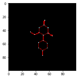
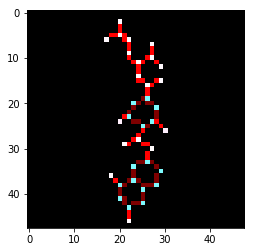
Nice. We can see the different atoms and bonds are coloured differently as they have different chemical information. Next step is to “chemcepterize” the entire collection of RDKit molecules and add a new column with the “images” to the dataframe
def vectorize(mol):
    return chemcepterize_mol(mol, embed=12)
data["molimage"] = data["mol"].apply(vectorize)
The dataset already had a split value indicating if it should be train or test set. The shape of the final numpy arrays are (samples, height, width, channels)
X_train = np.array(list(data["molimage"][data["split"]==1]))
X_test = np.array(list(data["molimage"][data["split"]==0]))
print(X_train.shape)
print(X_test.shape)
(609, 48, 48, 4)
(147, 48, 48, 4)
We also need to the prepare the values to predict. Here it is the IC50 for some DHFR inhibitors. The data is converted to log space and the robust scaler from scikit-learn is used to scale the data to somewhat between -1 and 1 (neural networks like this range and it makes training somewhat easier).
assay = "PC_uM_value"
y_train = data[assay][data["split"]==1].values.reshape(-1,1)
y_test = data[assay][data["split"]==0].values.reshape(-1,1)
from sklearn.preprocessing import RobustScaler
rbs = RobustScaler(with_centering=True, with_scaling=True, quantile_range=(5.0, 95.0), copy=True)
y_train_s = rbs.fit_transform(np.log(y_train))
y_test_s = rbs.transform(np.log(y_test))
h = plt.hist(y_train_s, bins=20)

Building the Chemception model
Now comes the interesting part where we will build the chemception network. For that we will use the Inception modules. These are interesting architectures. Instead of choosing/optimizing a convolutional kernel size, the modules split the data stream into three. The first tower is a recombination of the image channels/previous kernels with a convolution of 1, whereas the other two have kernel sizes of 3,3 and 5,5, respectively. The first tower is combined with a MaxPooling2D layer, whereas the others are combined with a prior 1 by 1 convolutional layer. This serves a dimension reduction by recombining the features from previous layers into a lower number of channels.
The first inception module is special, because I have removed the MaxPooling layer. The justification is that the features encoded in are not naturally ordered. Are positive charges more relevant than negatively charged? Is oxygen more important than carbon and nitrogen because it has a higher atomic weight? I think not, so I let the network figure it out with the first layer by recombining the channels, before I start to use the standard unit with max pooling.
After defining the Inception modules in some helper functions the network is build using Keras functional API, where the flow of Keras tensor objects is defined.
After the inception modules, I put a max pooling layer that spans the output of each kernel from the inception module, in a hope to create some features in the different kernels. We are interested if the features are present, but maybe not exactly where on the image. The output is flattened to one dimension and fed into a standard dense network with 100 neurons with the RELU activation function and a single output neuron with a linear activation function as we are aiming at a regression model.
In the end the computational graph is used with the model class, where the inputs and outputs are defined.
input_shape = X_train.shape[1:]
print(input_shape)
(48, 48, 4)
def Inception0(input):
    tower_1 = Conv2D(16, (1, 1), padding='same', activation='relu')(input)
    tower_1 = Conv2D(16, (3, 3), padding='same', activation='relu')(tower_1)
    tower_2 = Conv2D(16, (1, 1), padding='same', activation='relu')(input)
    tower_2 = Conv2D(16, (5, 5), padding='same', activation='relu')(tower_2)
    tower_3 = Conv2D(16, (1, 1), padding='same', activation='relu')(input)
    output = keras.layers.concatenate([tower_1, tower_2, tower_3], axis=-1)
    return output
def Inception(input):
    tower_1 = Conv2D(16, (1, 1), padding='same', activation='relu')(input)
    tower_1 = Conv2D(16, (3, 3), padding='same', activation='relu')(tower_1)
    tower_2 = Conv2D(16, (1, 1), padding='same', activation='relu')(input)
    tower_2 = Conv2D(16, (5, 5), padding='same', activation='relu')(tower_2)
    tower_3 = MaxPooling2D((3, 3), strides=(1, 1), padding='same')(input)
    tower_3 = Conv2D(16, (1, 1), padding='same', activation='relu')(tower_3)
    output = keras.layers.concatenate([tower_1, tower_2, tower_3], axis=-1)
    return output
input_img = Input(shape=input_shape)
x = Inception0(input_img)
x = Inception(x)
x = Inception(x)
od=int(x.shape[1])
x = MaxPooling2D(pool_size=(od,od), strides=(1,1))(x)
x = Flatten()(x)
x = Dense(100, activation='relu')(x)
output = Dense(1, activation='linear')(x)
model = Model(inputs=input_img, outputs=output)
print(model.summary())
__________________________________________________________________________________________________
 Layer (type) Output Shape Param # Connected to
 ==================================================================================================
 input_1 (InputLayer) (None, 48, 48, 4) 0
 __________________________________________________________________________________________________
 conv2d_1 (Conv2D) (None, 48, 48, 16) 80 input_1[0][0]
 __________________________________________________________________________________________________
 conv2d_3 (Conv2D) (None, 48, 48, 16) 80 input_1[0][0]
 __________________________________________________________________________________________________
 conv2d_2 (Conv2D) (None, 48, 48, 16) 2320 conv2d_1[0][0]
 __________________________________________________________________________________________________
 conv2d_4 (Conv2D) (None, 48, 48, 16) 6416 conv2d_3[0][0]
 __________________________________________________________________________________________________
 conv2d_5 (Conv2D) (None, 48, 48, 16) 80 input_1[0][0]
 __________________________________________________________________________________________________
 concatenate_1 (Concatenate) (None, 48, 48, 48) 0 conv2d_2[0][0]
 conv2d_4[0][0]
 conv2d_5[0][0]
 __________________________________________________________________________________________________
 conv2d_6 (Conv2D) (None, 48, 48, 16) 784 concatenate_1[0][0]
 __________________________________________________________________________________________________
 conv2d_8 (Conv2D) (None, 48, 48, 16) 784 concatenate_1[0][0]
 __________________________________________________________________________________________________
 max_pooling2d_1 (MaxPooling2D) (None, 48, 48, 48) 0 concatenate_1[0][0]
 __________________________________________________________________________________________________
 conv2d_7 (Conv2D) (None, 48, 48, 16) 2320 conv2d_6[0][0]
 __________________________________________________________________________________________________
 conv2d_9 (Conv2D) (None, 48, 48, 16) 6416 conv2d_8[0][0]
 __________________________________________________________________________________________________
 conv2d_10 (Conv2D) (None, 48, 48, 16) 784 max_pooling2d_1[0][0]
 __________________________________________________________________________________________________
 concatenate_2 (Concatenate) (None, 48, 48, 48) 0 conv2d_7[0][0]
 conv2d_9[0][0]
 conv2d_10[0][0]
 __________________________________________________________________________________________________
 conv2d_11 (Conv2D) (None, 48, 48, 16) 784 concatenate_2[0][0]
 __________________________________________________________________________________________________
 conv2d_13 (Conv2D) (None, 48, 48, 16) 784 concatenate_2[0][0]
 __________________________________________________________________________________________________
 max_pooling2d_2 (MaxPooling2D) (None, 48, 48, 48) 0 concatenate_2[0][0]
 __________________________________________________________________________________________________
 conv2d_12 (Conv2D) (None, 48, 48, 16) 2320 conv2d_11[0][0]
 __________________________________________________________________________________________________
 conv2d_14 (Conv2D) (None, 48, 48, 16) 6416 conv2d_13[0][0]
 __________________________________________________________________________________________________
 conv2d_15 (Conv2D) (None, 48, 48, 16) 784 max_pooling2d_2[0][0]
 __________________________________________________________________________________________________
 concatenate_3 (Concatenate) (None, 48, 48, 48) 0 conv2d_12[0][0]
 conv2d_14[0][0]
 conv2d_15[0][0]
 __________________________________________________________________________________________________
 max_pooling2d_3 (MaxPooling2D) (None, 1, 1, 48) 0 concatenate_3[0][0]
 __________________________________________________________________________________________________
 flatten_1 (Flatten) (None, 48) 0 max_pooling2d_3[0][0]
 __________________________________________________________________________________________________
 dense_1 (Dense) (None, 100) 4900 flatten_1[0][0]
 __________________________________________________________________________________________________
 dense_2 (Dense) (None, 1) 101 dense_1[0][0]
 ==================================================================================================
 Total params: 36,153
 Trainable params: 36,153
 Non-trainable params: 0
 __________________________________________________________________________________________________
 None
In the end the model ends up not having a terrible lot of parameters, only 36.153, which is a lot lower than others I have trained on even smaller datasets. This is because I have lowered the number of kernels for each tower from 64 to 16, as I judge the dataset to be rather small. The images may be a lot simpler than, say, photos of cats, so it may work anyway.
For the optimization I use the Adam optimizer and the mean squared error as a loss function.
optimizer = Adam(lr=0.00025)
model.compile(loss="mse", optimizer=optimizer)
The next part is crucial to avoid overfitting. Here the ImageDataGenerator object is used to perform random rotations and flips of the images before the training as a way of augmenting the training dataset. By doing this, the network will learn how to handle rotations and seeing the features in different orientations will help the model generalize better. Not including this will lead to completely overfit models. We have not encoded stereochemical information in the images, otherwise the flipping should be done by other means.
The training set is concatenated to 50 times the length to have some sensible size epochs.
from image import ImageDataGenerator
generator = ImageDataGenerator(rotation_range=180,
                               width_shift_range=0.1,height_shift_range=0.1,
                               fill_mode="constant",cval = 0,
                               horizontal_flip=True, vertical_flip=True,data_format='channels_last',
                               )
#Concatenate for longer epochs
Xt = np.concatenate([X_train]*50, axis=0)
yt = np.concatenate([y_train_s]*50, axis=0)
batch_size=128
g = generator.flow(Xt, yt, batch_size=batch_size, shuffle=True)
steps_per_epoch = 10000/batch_size
Training the Chemception model
Now for the interesting part: Training. To lower the learning rate once the validation loss starts to plateau off I use the ReduceLROnPlateau callback avaible as part of Keras.
reduce_lr = ReduceLROnPlateau(monitor='val_loss', factor=0.5,patience=10, min_lr=1e-6, verbose=1)
history = model.fit_generator(g,
                              steps_per_epoch=len(Xt)//batch_size,
                              epochs=150,
                              validation_data=(X_test,y_test_s),
                              callbacks=[reduce_lr])
Epoch 1/150
 237/237 [==============================] - 31s 131ms/step - loss: 0.1241 - val_loss: 0.1208
 Epoch 2/150
 237/237 [==============================] - 28s 119ms/step - loss: 0.1135 - val_loss: 0.1068
 Epoch 3/150
 237/237 [==============================] - 28s 119ms/step - loss: 0.1123 - val_loss: 0.1071
 Epoch 4/150
.....
237/237 [==============================] - 29s 122ms/step - loss: 0.0362 - val_loss: 0.0361
 Epoch 150/150
 237/237 [==============================] - 29s 122ms/step - loss: 0.0355 - val_loss: 0.0360
Models can be saved and loaded. The history objects history dictionary is pickled.
name = "Chemception_std_notebook_demo"
model.save("%s.h5"%name)
hist = history.history
import pickle
pickle.dump(hist, file("%s_history.pickle"%name,"w"))
#from keras.model import load_model
#model = load_model("%s.h5"%name)
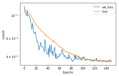
The convergence of the training can be judged from a plot of the learning process. Somewhat unusual, when theres no regularization: The validation loss drops before the loss. The validation set is not augmented and thus consists of some “perfect” pictures, whereas maybe it may take the network some longer to deal with all the rotations, which also introduces some pixel artifacts due to the low resolution.
for label in ['val_loss','loss']:
    plt.plot(hist[label], label = label)
plt.legend()
plt.yscale("log")
plt.xlabel("Epochs")
plt.ylabel("Loss/lr")
Plotting and Evaluating the Performance
y_pred_t = rbs.inverse_transform(model.predict(X_train))
y_pred = rbs.inverse_transform(model.predict(X_test))
plt.scatter(np.log(y_train), y_pred_t, label="Train")
plt.scatter(np.log(y_test), y_pred, label="Test")
plt.xlabel("log(PC_uM)")
plt.ylabel("predicted")
plt.plot([-10,6],[-10,6])
plt.legend()
corr2 = np.corrcoef(np.log(y_test).reshape(1,-1), y_pred.reshape(1,-1))[0][1]**2
rmse = np.mean((np.log(y_test) - y_pred)**2)**0.5
print("R2 : %0.2F"%corr2)
print("RMSE : %0.2F"%rmse)
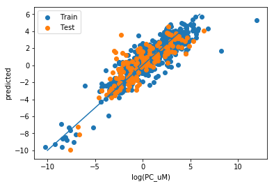
R2 : 0.67
RMSE : 1.50
This looks very similar to the performance I have obtained with this dataset previously with other means.
Visualizing the Layers
It can be interesting to try and understand how the model “sees” the molecules. For this I’ll take an example molecule and plot some of the outputs from the different layers. I’ve taken the compound with the lowest IC50, number 143 in the dataset.
molnum = 143
molimage = np.array(list(data["molimage"][molnum:molnum+1]))
mol = data["mol"][molnum]
The molecule looks like this
from rdkit.Chem import Draw
Draw.MolToImage(mol)
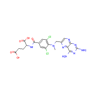
And has this “chemcepterized” image as shown below
plt.imshow(molimage[0,:,:,:3])
The first example is the third layer, which is the 1,1 convolution which feeds the 3,3 convolutional layer in tower 2.
layer1_model = Model(inputs=model.input,
                    outputs=model.layers[2].output)
kernels1 = layer1_model.predict(molimage)[0]
def plot_kernels(kernels):
    fig, axes = plt.subplots(2,3, figsize=(12,8))
    for i,ax in enumerate(axes.flatten()):
        ax.matshow(kernels[:,:,i])
        ax.set_title("Kernel %s"%i)
plot_kernels(kernels1)
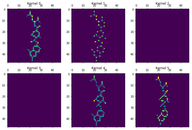
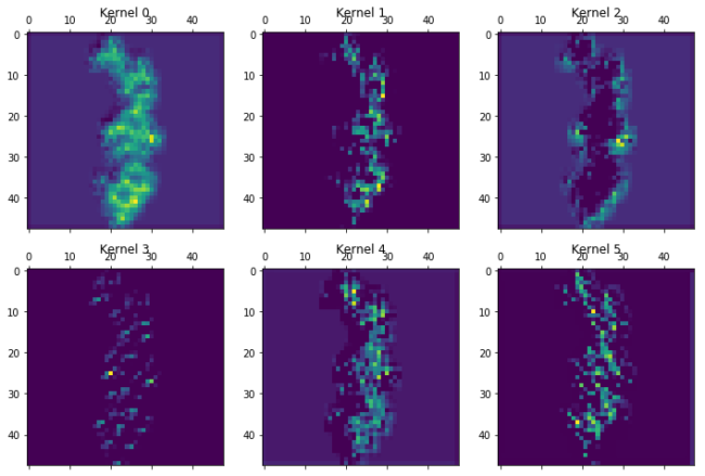
The different kernels (here the first 6 out of 16), have already recombined the information in Chemception image. Kernel 5, seem to focus on bonds, as it has removed the bond information when there were atoms in the other layers. Kernel 1 focuses on atoms and is most activated for aliphatic carbon. Kernel 4 is most exited with the chlorine atoms, but also contain bond information. Kernel 2 and 3 seems empty. Maybe they are activated by other molecules on features not present in the current molecule, or maybe they were unneeded. Lets go deeper…..
for layer in [7,13,15,19,20]:
    print("Layer %i"%layer)
    plot_kernels(Model(inputs=model.input,outputs=model.layers[layer].output).predict(molimage)[0])
    plt.show()
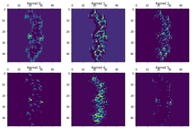
Layer 7
Layer 13
Layer 15
Layer 19
Layer 20
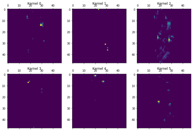
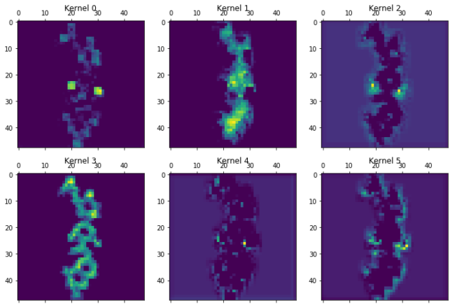
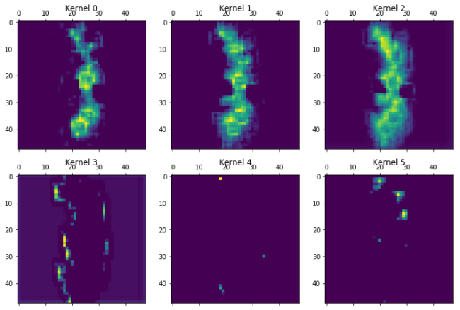
A generel trend as we go through the layers is the more and more abstract and specific features that are created. The chlorine atoms seem to light up in a lot of the kernels, but others focus on other features. Kernel 0 to 2 in layer 19 seem to focus on all that is not the chlorine atoms. Kernel 5 in the same layer activates near the double bonded oxygens. The last layer just before the total kernel-wise max pooling only seem to focus on very specific parts of the molecule. Kernel 0 could be the amide oxygen. Kernel 2 and 5 the chlorine atoms. Kernel 4 seem to like the double bonden oxygens, but only from the carboxylic acid groups, not the amide. Kernel three gets activated near the terminal carboxylic acid’s OH. These are only the first 6 of the features that are extracted from the images and fed forward to the dense layer.
Summary
In this blog-post I have shown how to create a chemception model with a few lines of python code using RDKit for the chemistry and Keras for the neural networks. The Sutherland DHFR dataset is very dependant on the classes of molecules in there, and the random division of the classes into the train and test set do not show if these kind of chemception models can carry any transfer of the SAR from class to class, or they merely recognize the compound class and assigns an average IC50. If you do happen to recreate a Chemception model and make a division based on classes for the train and test sets, let me know how the performance was in the comments below.
Hi Esben, this looks really interesting. Have you tried using a similar approach in a variational auto-encoder to get a latent space representation? This could be of interest to have the algorithm dream up new molecules directly from drawings — thus getting rid of some of the problems around SMILE representation.
Also using this with approaches such as grad-cam and similar, are you able to show which features of the molecule / drawing are most important for a given prediction. This would be interesting within a chemical series to see which areas lights up for particular assay read-outs.
Hi Troels,
Good to hear from you. Hope everything is fine in Boston.
I have thought about using this representation as a base for auto-encoders, but haven’t had the time to experiment yet, and yes, it also opens up some interesting possibilities for mapping the importance. Let me know your results if you try it yourself.
Best Regards
Esben
I get this error
ArgumentError: Python argument types in
rdkit.Chem.rdPartialCharges.ComputeGasteigerCharges(Mol)
did not match C++ signature:
ComputeGasteigerCharges(RDKit::ROMol const* mol, int nIter=12, bool throwOnParamFailure=False)
when I run
mol = data[“mol”][0]
v = chemcepterize_mol(mol, embed=10, res=0.2)
print(v.shape)
plt.imshow(v[:,:,:3])
I’m not sure how to fix this. Is this a rdkit error?
I would check that mol is a proper RDKit molecule or NoneType. If RDKit can’t sanitize the molecule when parsing SMILES or reading SD files, it returns None instead of failing.
Thanks! This is such a great blog!
You’r welcome. Let me know how your chemical deep learning work out 😉
What was the SMILES string for the molecule you used? I am still getting errors when I try to chemcepterize.
AttributeError: ‘str’ object has no attribute ‘ToBinary’
You have a string, not an RDKit mol! Is it the smiles?
mol = rdkit.Chem.MolFromSmiles(smiles)
check the type. e.g. type(mol)
Yes, it’s a SMILES string I got from Chembl. I’m still getting errors about C++ checksums…
Here’s my file:
smiles PC_uM_values
NC(=O)[C@@H]1CCCN1C(=O)[C@H](CC1=CNC=N1)NC(=O)[C@@H]1CCC(=O)N1
CCCCC(=O)OCC(=O)[C@H]1[C@H](C)C[C@H]2[C@@H]3C[C@H](F)C4=CC(=O)C=C[C@]4(C)[C@@]3(F)[C@@H](O)C[C@]12C
NC(=O)C1CSCN1C(=O)C(CC1=CN=CN1)NC(=O)C1CCCC(=O)N1
NC(=O)C1CCCN1C(=O)C(CC1=C(I)N=C(I)N1)NC(=O)C1CCC(=O)N1
CC1SC=C(NC1=O)C(=O)NC(CC1=CN=CN1)C(=O)N1CCCC1C(N)=O
NC(=O)C1CSCN1C(=O)C(CC1=CN=CN1)NC(=O)C1CCCC(=O)N1
NC(=O)C1CCCN1C(=O)C(CC1=C(N=CN1)[N+]([O-])=O)NC(=O)C1CCC(=O)N1
CC1CCN(C1C(N)=O)C(=O)C(CC1=CN=CN1)NC(=O)C1CCC(=O)N1
NC(=O)C1CCCN1C(=O)C(CC1=C(I)N=C(I)N1)NC(=O)C1CCC(=O)N1
NC(=O)C1CCCN1C(=O)C(CC1=C(N=CN1)[N+]([O-])=O)NC(=O)C1CCC(=O)N1
CC1CCN(C1C(N)=O)C(=O)C(CC1=CN=CN1)NC(=O)C1CCC(=O)N1
CC1(C)CCN(C1C(N)=O)C(=O)C(CC1=CN=CN1)NC(=O)C1CCC(=O)N1
CC1(C)CCN(C1C(N)=O)C(=O)C(CC1=CN=CN1)NC(=O)C1CCC(=O)N1
You need to convert to RDKit molecule objects and check that the conversion went OK, before you attempt to use the chemcepterize_mol function. See my first reply.
I tried converting aspirin and a couple other molecules into RDKIt molecule objects and I’m still getting the same errors…. I might try it again on another computer with rdkit and anaconda properly installed. I’m getting a bunch of system errors… 🙁
Thanks!
Hi,
I have an issue with the following lines of code which result in an error.
###############################################
def vectorize(mol):
return chemcepterize_mol(mol, embed=12)
data[“molimage”] = data[“mol”].apply(vectorize)
################################################
ERROR:
IndexError: index 49 is out of bounds for axis 0 with size 48
I tried to apply for loop but coudn’t succeed as given in the link below.
https://stackoverflow.com/questions/52988278/how-to-store-an-image-in-pandas-dataframe-column
Your molecules are probably too large for the embedding. Try and raise the embed parameter.
Thank you.
A quick question, you applied the RobustScaler to the y_train because the problem under consideration was regression problem?
I apply the RobustScaler to get the output values somewhere in the range -1 to 1. Training works best then. I think it is due to weight initialization schemes, optimizers, gradients, error sizes etc. are developed and optimized together to work in that range.
In my case the shape of the data is different.
###################################
print(np.shape(X_train))
4554
###########################
I have 4554 images. It is not giving me the shape like (m,w,h,c).
When I print the shape of first dimension, it shows the shape as follows.
#####################################################
X_train[0].shape
(120, 120, 4)
#############################################
How can I get my data in the same shape as in your example. (4554,120, 120, 4)?
Oh, I resolved the issue.
Thanks. I was splitting the data in a different way, which caused the dimension problem.
From your description it seems like you have an array of objects that are maybe arrays. The casting from a list in this line X_train = np.array(list(data[“molimage”][data[“split”]==1])) may not work due to library version differences.
Maybe try to cast the values e.g. something like
X_train = np.array(data[“molimage”][data[“split”]==1].values)
or maybe .reshape() can be your friend.
Hi,
Are the images created in data[“molimage”] 8 bit images? OR what is the bit size of each pixel?
Can we do normalization of the input images in this case?
Hi,
great post! I don’t have any experience with CNNs yet, therefore I would like to ask what kind of hyperparameters must be adjusted in this type of network? From your post, I assume that you tried only one combination. Is this sufficient?
The second question is about the 2D image generation. You state that you performed random rotations and flips of the images and that was sufficient because you didn’t include any stereospecific information. Isn’t it true that some molecules can have alternative 2D projections (I am not referring to enantiomerism or cic-trans isomerism)? For example, the following ethyl phenyl sulfide can be projected to 2D in two ways, the first is as shown in the following image in which the ethyl points to the right and the second possible way (not shown) is when the ethyl points to the left.
https://www.sigmaaldrich.com/content/dam/sigma-aldrich/structure0/175/mfcd00009265.eps/_jcr_content/renditions/mfcd00009265-medium.png
Shouldn’t you also take into consideration such cases when you generate alternative image representations of the same molecule?
Hi Thomas,
Thank you for commenting and Merry Christmas. There’s tons of hyperparameters and things to tune with artificial neural networks, but for this specific architecture, the number of kernels used in the towers is probably an important setting. I tuned it down from the default used in Inception networks used for image recognition in lieu of the small dataset used for training, but addition of dropout layers is also an often used way to counteract over-fitting.
As for your second question, I never stated that the data augmentation is optimal. The lack of stereo information makes it possible to use flips, otherwise the stereo information needed to be handled explicitly as you can’t just flip the 2D coordinates without also adjusting the stereo. As for your suggestion, it could indeed be possible to add 2D conformational sampling as an extra form of data augmentation and maybe juice out a bit extra performance from the approach. To my knowledge it has not been tried or reported, so there’s possibly a nice small project/publication there if you have the time or special expertise regarding calculation of 2D coordinates. Let me know if you want to discuss it further 😉
The approach as presented in the simple form here, works surprisingly well and is a good example of the automatic feature extraction/generation from a simple embedding that can be had with a deep learning approach.
BR
Esben
Hi Esben,
Merry Christmas to you, too. My example was incorrect because by image flipping you can get both alternative 2D depictions. In the following example flipping does not give the alternative 2D representation:
https://github.com/tevang/tutorials/blob/master/2D_conformation_sampling/alternative_2D_projections.png
On second thought, cis-trans isomerism could be also considered to augment the training set.
Ideally, there should have been only one 2D representation for each molecule and compounds within each chemical series should have had the common atoms in the same orientation. I see that you use rdkit.Chem.rdDepictor.Compute2DCoords(). Maybe, GenerateDepictionMatching2DStructure() or GenerateDepictionMatching3DStructure() could be better, given special treatment of similar compounds. It could also be good to start from a unique SMILES representation for each compound – although I am not sure if this is possible. Have you tried DeepSMILES (https://github.com/nextmovesoftware/deepsmiles)? I must think more about these ideas and discuss them with other people. Maybe I could find a student to work on this.
But I am afraid that his problem boils down to correct binding pose prediction, which is extremely challenging to tackle for large datasets. In my hands, 3D feature vectors (3D pharmacophores, 3D shape and charge distribution vectors, per-residue contribution to the free energy of binding) worked well only when the input conformation was the correct binding pose (not the lowest energy conformer as others claim). They also tended to have worse performance than 2D fingerprints, probably due to wrong binding poses for some of the compounds. This is the reason why I haven’t touched CNNs yet. However, in the new year, I am planning to experiment with more complicated architectures than the MLPs that I currently use.
What is currently your employment status? Will you be able to continue on your old projects?
BW
Thomas
Hi,
Yes your example could maybe be handled by the flipping, but I understood what you meant. I have also previously been disappointed by 3D fingerprints, but maybe its time to revisit with the “deep learning” glasses on. Generally the variation is handled via data augmentation and simulation of noise/irrelevant variation rather than normalizing efforts. Your cat aligning algorithm will take a lot longer and be a lot harder for you to program than letting your GPU train a more complex network, but maybe in the binding pose/conformer case its the way to go.
I’ve just started working at Astrazeneca in Sweden, so I’m quite busy starting up the projects here (But I will find time for a chat if you are interested in discussing this further). AZ and our group are quite open for scientific collaborations, secondment etc. but I’m still figuring that out.
Best Regards
Esben
Hello Esben,
I will contact you by email by the end of this month to talk about this and about something else that I have thought that involves also NMR.
Best wishes,
Thomas
Would it be possible to provide the exact file used including the splits? In my case it doesn’t even come close to building a nice model and I simply copy&pasted the code. Only difference might be the dataset. I used the on form your github:
https://github.com/EBjerrum/SMILES-enumeration/blob/master/Example_data/Sutherland_DHFR.csv
And of course the used split is different albeit histogram looks the same.
For me this is absolutely NOT reproducible with above data. I advise anyone to try themselves before trying on your own data set.
Hi Thomas,
Sorry to hear you are struggling to train a model. I’ll try and dig out the dataset I used and also how the splits were made from my previous workstation. Either there were some splits provided by the original data from the Sutherland paper or I probably split the dataset random (sklearn.model_selection.train_test_split). I usually pre-split the dataset and save the splits when I process the datasets as this makes it easier to compare across different models. There’s also an uncertainty on the estimation of R2 and other metrics which is surprisingly high, Patrick Walters have a nice blog-post explaining that: https://practicalcheminformatics.blogspot.com/2018/09/predicting-aqueous-solubility-its.html
How did you do your splitting? How bad is your model performance?
There’s a couple of compound series/classes in the dataset, and if they are unevenly divided between the train and test splits the model will maybe not give as nice statistics. Its actually a good way to test the applicability domain and generalization of a model to make a class based split.
Looking over my old data preparation scripts, there were a detail which can be crucial. The dataset contains signed values (like “>42”), and I divided the dataset into “dirty” points (> signed) and “clean” (value as is). Using the assumption that the uncertainty on the “clean” values is lower, the datasets clean points were used for random splitting into a train and test set. The dirty points were then joined into the train set only. There was also an outlier with what looks like a factor 1000 error, but that was left “as-is”. Maybe I should write a blog post about it, thanks for the inspiration. I re-exported and uploaded the .h5 file to https://github.com/EBjerrum/SMILES-enumeration/blob/master/Example_data/Sutherland.h5
Thanks for your prompt reply. I did retry with the data file you provided. (Hint for others that want to try, the id in the h5 file is “table” and not “Data” like in code above).
I copy pasted your code 1:1 into a Jupyter Notebook but fail to reproduce the results:
R2 : 0.45
RMSE : 2.03
But that is only one point. The network fails to really improve after around epoch 20 and a validation loss of around 0.06.
Only difference is RDKit, Keras and tensorflow versions but that theoretically shouldn’t lead to such huge differences.
As a completely different topic I also wonder if normalization needs to be applied since each layer has completely different ranges especially the atom number layer.
Well I fail to understand what it is that make it now work for you, you have some signal, but not a lot. But yes, normalization could be a good thing, If you try, let us know the results in the comments. Today I actually use another embedding for the atom types than the atom number, but this was the original schema from the Goh paper. The blog post here is kept as simple as possible and is meant as a starting point for your own further experimentation, not production ready and robust code.
hello, line 9,mol.GetBonds() or cmol.GetBonds()?, is that matter???
Hi, Good catch. It should be cmol.GetBonds() for consistency. But as the bond information is the same in mol and cmol, it will not matter much I think.
Nice coding but when I was going to run it, I encountered a problem.
I have a problem to activate tensorflow and rdkit in anaconda win 10 but when one of them are activate the another is not working and so on!
Do you know what is my problem? What about the versions of python?tensorflow?rdkit? anaconda? that works well for you.
I don’t use win 10, so I don’t know whats your precise issue. However, I think you must build your own Conda environment with both RDKit and tensorflow. Start with RDKit, then conda install the rest from there.
Dear Esben
I am completely new to machine learning. I have used the code exactly as is with a few minor modifications for version updates etc. The code executes without any problems but unfortunately I cannot reproduce the performance of the model as shown. The val-loss curve seems to plateau at 6*10E-2. To complete 150 epochs takes 2 full days on my Linux work station. I am currently changing the learning rate to a bigger value of 0.001.
Your val_loss seem a bit higher than the one I achieved. Its a good idea to try and adjust the learning. Either up or down. I think I originally had to adjust down a bit. Your training time seems very slow. Are you using a GPU? If not, get one or get it working.
Hi Esben. Thanks for your advice. We plan to buy a GPU in the near future.
I made several changes to try and improve the performance of my implementation of the network.
(I) I ran for only 20 epochs. Thomas Struntz also noted that after 20 epochs there was no apparent improvement. Also I have access to limited computing resources.
Secondly I changed the learning rate for Adam to 0.001 as this seems to be the recommended default for Adam with Keras.
Thirdly I additionally used mae as an optimizer as you mentioned potential outliers in your blog, and mae is less impacted by having a few molecules with potentially misleading data values.
The combination of these settings lead to much improved loss/validation-loss curves. There was no longer any indication of overfitting and pretty good convergence, though the model with rmse as the optimizer looked as it needs more epochs to converge properly.
MAE rsquared of 0.56 and rmse 1.74
rmse rsquared 0.51 and rmse 2.08
These are not as good as your original values but now seem to be heading in the right direction.
There are several things that I find a bit confusing. The rmse optimizer gives a smaller loss from its curves but mae gives a better rsquared. Is the purpose of the validation-loss curve then just to highlight potential problems with the model ?
Secondly, now that I have done this as a practical exercise, I am now not sure what happens during the validation step. During training the weights and biases are optimized. Are the parameters also tweaked in some way during the validation step ?
As a general comment I am enthralled by the pictorial representation of molecules. I come from a traditional QSAR and pharmacophore background where there are often alignment issues for molecules containing diverse structures. This approach seems to have the potential to be informative and bypass alignment issues.
However, do you think it could eventually be possible to create common pharmacophores from these isolated features coming from different chemotypes ?
Good to hear that you are making progress. Most of my training/blog posts are done using a GTX 1060 with 6 GB of ram, which are quite affordable nowadays. The loss of mae and mse are not the same and can not be compared, Huber loss is an intermediate outlier tolerant loss function, which are mse close to zero but turns linear rather than exponential at higher error. It could also be a smart idea to look for and remove outliers before training. And no single metric captures all aspects of the model, so both RMSE and linearity should be investigated. The validation loss curve is good to find potential overfitting issues and sometimes can be useful to pick an early stopping (goes down and then up as overtraining/overfitting appears). No updates of the weights should happen during validation, but you do turn off regularization such as dropout which are only active during the training phase. This can lead to the interesting situation where the training loss is higher than the validation loss.
Is it possible to adapt the code to add the features to larger molecules? I tried to filter my dataset to have SMILES codes shorter than 70 but still I have to increase the embedding or decrease the resolution by a lot, and the resulting image is large with just the molecule in the middle (which I can barely see).
Yes some of them must look small, but you’ll probably have some large molecules in your dataset, or why do you otherwise have to increase the embedding. Lowering resolution beyound the point where atoms are seperated with bonds, may not be successful.
I had run the whole code perfectly. i have one question… As the data is already is split into train and test. But where is the class label defined for each train and test
It’s a regression problem, so there should be a column with the activity values in there. If you want to make a classifier, you’d have to adapt the output dense neuron to have a sigmoid activation function and use binary cross-entropy, and then create your own classes based on cut-offs of the activity values.
Hello! Thank you for this awesome post. I was wondering if there was a way to get the SMILES strings of the chemcepterized representations or if they can be directly converted into a 2D molecule drawing. Can you think of some ways that might be possible?
Hi Varsha,
I haven’t made any explicit code that does just that. Seems like it would be non-trivial to do by hand. Alternatively a deep learning solution can be made. I did some experiments going from chemception image to SMILES strings as a minor part of the publication: Bjerrum, Esben, and Boris Sattarov. “Improving Chemical Autoencoder Latent Space and Molecular De Novo Generation Diversity with Heteroencoders.” Biomolecules 8.4 (2018): 131.
It seems to reach a high reconstructability. The basic idea is that you read in the image in a chemception network, but then connects the output max-pool layer to dense layers that set the initial states of an RNN that reconstructs the SMILES. After generation of a lot of chemcepterized images from SMILES the network can be trained to do the inverse task as you want. Please let me know if you get it to work or find another way.
I will surely look into the RNN based model. Great paper on the heteroencoders by the way. Thank you for all your insights.
PS: I didn’t get the email for confirmation of subscription.
Thanks for the feedback about the mail, I’ll look into it when time allows
Hi Esben,
Can you please list out what needs to be done in this code in order for getting publication.
in terms of image augmentation, number of layers or what else need to be added in layers other than bonds, bond order, atomic number, Gasteiger charges and hybridization..
As I am working on this but is based on classification.
The question is kind of too general to answer well. You need to adapt the code to your problem, get some good results and write a publication
Hi Esben,
In this case, why didn’t you normalize an image by dividing by 255? dividing by 255 is very common.
Thanks for commenting. If you make a histogram over the values in a chemception image, and from, say, mnist, you’ll see the distribution of values are very different.
I see. So you did standardize value based on the histogram. May I ask in case I had never seen this case before, would scaling input by diving by 255 still be acceptable?
No I didn’t standardize. Most values are zero, and the rest are usually pretty low.
Dear Esben
I hope you can see this message!
Thanks for this awesome post! But when I was going to run code on the other one data set, I encountered a problem:
the loss and val_loss quicky become NAN in Epoch 1. the data set include 1300 molecule with relevant SMILES and pLC50 (mol/L). min value = 0.36, max value = 9.53 mean value = 4.23 and stddev=1.13.
To resolve my question, I have tried 2mthods but no effects: 1. check the data to ensure no NAN value; 2. reduce learing rate from 0.00025 to 0.00005. could you help me?
I have also some questions during learn CNN-Regression:
1. Does the significant digit affect the performance of the regression model?In other words, the longer the number of bits, the harder it is to fit?
2. some bolgs say that loss function “msle” is better than “mse” when I using “msle” as loss fuction, the loss function declines and enters the smoothing period, but “rmse” and “mae” is higher than the results of Multiple linear regression.
3. when I add Btach-Nmormalization behind of conv2d layers, the the loss function curve becomes like an electrocardiogram, hard to converge 🙁
Looking forward to your reply!
Hi Wang Liu,
Thanks for the questions and interest in my old blog-post. I can understand that you are not using the dataset as in the example, so some adaptation of the hyperparameters are probably needed. Moreover, Keras has developed, so this old code may need a bit of updating. NAN loss means that training is unstable, and that could be counteracted by tuning the learning rate and/or increasing the batch size. You could do a bayesian optimisation of these two hyperparameters with e.g. optuna or hyperopt. I have another old blogpost about that Tune your deep tox neural network with free tools. As for your specific questions: @1. No, I wouldnt expect so. The signa from the loss function is not really changed a lot with a different number of significant digits, i.e. (1-0.5)**2 = 0.25 is not very different and with a different sign than (1,000001−0.5)^2 = 0,250001. @2. I haven’t experimented with msle, but from your description the influence on the metrics, it sounds like it works worse in your case. Have you also checked the correlation coefficient of the regression? @3. Yes, batch normalization doesn’t work here. I think it is due to the images being all artificial and the background is all padding with 0, so the pixel distribution is far from normal.
Please come back and give an update if you make it work, and what made it work for you.
Best Regards
Esben