A deep Tox21 neural network with RDKit and Keras

Esben Jannik Bjerrum/ January 15, 2017/ Blog, Cheminformatics, Machine Learning, Neural Network, RDkit/ 15 comments

I found some interesting toxicology datasets from the Tox21 challenge, and wanted to see if it was possible to build a toxicology predictor using a deep neural network. I don’t know how many layers a neural network actually has to have to be called “deep”, but its a buzz word, so I’ll use it ;-). The idea and hope of deep learning is to let the network learn a hierarchy of more and more abstract concepts by passing it sequentially through layers of neurons, where one layers output are used as input to the next. They can be training in a supervised fashion via the back propagation algorithm, which updates the weights based on the mistakes the network makes when it tries to predict labeled samples. In the end of the blog post I’ll compare the performance of the deep neural network with a more simple logistic regression model with regularization.
Deep networks are prone to over fitting as the number of parameters in the network quickly adds up. In this example network I use a Morgan Circular fingerprint with 8192 bits and three fully connected dense layers as well as a single output neuron. The first layer will have 8192*80 connections to it, the next 80*80 and so forth, so the total number of weights that needs fitting is 668240. This is way past the number of available samples in the Tox21 datasets, so overfitting is likely.
Luckily there are ways to balance the bias/variance by means of regularization. By adding a penalty for high weights, the network can be forced to use smaller weights and many small contributions, instead of balancing of large weights with opposite signs to get the prediction of the train set 100% correct. I have covered the use of L2 regularization in a previous blogpost. Another regularization technique for neural network is dropout. Here a percentage of the activations are randomly dropped between layers during the training phase of the network. This makes it more difficult for the network to let the output of the neurons depend to much on the output of the others and breaks the dependence between the neurons. This should lead to single neurons doing more generalized work. The Tox21 dataset is in the range of a few thousands, so both techniques are used in the example below.
Enough of the talking, lets see the code. First a bunch of imports.

#Pandas and Numpy
import pandas as pd
import numpy as np
#RDkit for fingerprinting and cheminformatics
from rdkit import Chem, DataStructs
from rdkit.Chem import AllChem, rdMolDescriptors
#MolVS for standardization and normalization of molecules
import molvs as mv
#Keras for deep learning
from keras.models import Sequential
from keras.layers import Dense, Dropout
from keras.callbacks import ReduceLROnPlateau
from keras.regularizers import WeightRegularizer
from keras.optimizers import SGD
#SKlearn for metrics and datasplits
from sklearn import cross_validation
from sklearn.metrics import roc_auc_score, roc_curve
#Matplotlib for plotting
from matplotlib import pyplot as plt

The dataset was downloaded from https://tripod.nih.gov/tox21/challenge/data.jsp and converted to CSV files with pandas and RDKit, here exemplified with the training data.

#!/usr/bin/python
from rdkit import Chem
import pandas as pd
filename = "tox21_10k_data_all.sdf"
basename = filename.split(".")[0]
collector = []
sdprovider = Chem.SDMolSupplier(filename)
for i,mol in enumerate(sdprovider):
	try:
		moldict = {}
		moldict['smiles'] = Chem.MolToSmiles(mol)
		#Parse Data
		for propname in mol.GetPropNames():
			moldict[propname] = mol.GetProp(propname)
		collector.append(moldict)
	except:
		print "Molecule %s failed"%i
data = pd.DataFrame(collector)
data.to_csv(basename + '_pandas.csv')

 
 
During this challenge, there was a training set, a test set for the leader board, and a secret set for finding the winners. I reuse these sets as training, validation and test set respectively.

#Read the data
data = pd.DataFrame.from_csv('tox21_10k_data_all_pandas.csv')
valdata = pd.DataFrame.from_csv('tox21_10k_challenge_test_pandas.csv')
testdata = pd.DataFrame.from_csv('tox21_10k_challenge_score_pandas.csv')

The molecules were with salt forms, so they were standardized and normalized to the parent molecular form with MolVS.

#Function to get parent of a smiles
def parent(smiles):
 st = mv.Standardizer() #MolVS standardizer
 try:
  mols = st.charge_parent(Chem.MolFromSmiles(smiles))
  return Chem.MolToSmiles(mols)
 except:
  print "%s failed conversion"%smiles
  return "NaN"
#Clean and standardize the data
def clean_data(data):
 #remove missing smiles
 data = data[~(data['smiles'].isnull())]
 #Standardize and get parent with molvs
 data["smiles_parent"] = data.smiles.apply(parent)
 data = data[~(data['smiles_parent'] == "NaN")]
 #Filter small fragents away
 def NumAtoms(smile):
  return Chem.MolFromSmiles(smile).GetNumAtoms()
 data["NumAtoms"] = data["smiles_parent"].apply(NumAtoms)
 data = data[data["NumAtoms"] > 3]
 return data
data = clean_data(data)
valdata = clean_data(valdata)
testdata = clean_data(testdata)

The fingerprints were calculated with the excellent RDkit library.

#Calculate Fingerprints
def morgan_fp(smiles):
 mol = Chem.MolFromSmiles(smiles)
 fp = AllChem.GetMorganFingerprintAsBitVect(mol,3, nBits=8192)
 npfp = np.array(list(fp.ToBitString())).astype('int8')
 return npfp
fp = "morgan"
data[fp] = data["smiles_parent"].apply(morgan_fp)
valdata[fp] = valdata["smiles_parent"].apply(morgan_fp)
testdata[fp] = testdata["smiles_parent"].apply(morgan_fp)

The dataset is converted into numpy arrays. I choose the SR-MMP property. This is the result of an cellular stress response assay measuring disturbance of the mitochondrial membrane potential. Theres no particular reason I chose this, just the first one I tried.

#Choose property to model
prop = 'SR-MMP'
#Convert to Numpy arrays
X_train = np.array(list(data[~(data[prop].isnull())][fp]))
X_val = np.array(list(valdata[~(valdata[prop].isnull())][fp]))
X_test = np.array(list(testdata[~(testdata[prop].isnull())][fp]))
#Select the property values from data where the value of the property is not null and reshape
y_train = data[~(data[prop].isnull())][prop].values.reshape(-1,1)
y_val = valdata[~(valdata[prop].isnull())][prop].values.reshape(-1,1)
y_test = testdata[~(testdata[prop].isnull())][prop].values.reshape(-1,1)

Now for the more interesting part. Building the neural net with Keras and train it. First layer is a dropout layer, so 20% of the incoming features are randomly dropped. Then follows three dense layers with both 50% and weight regularization. The last layer is a single neuron with sigmoid activation function.
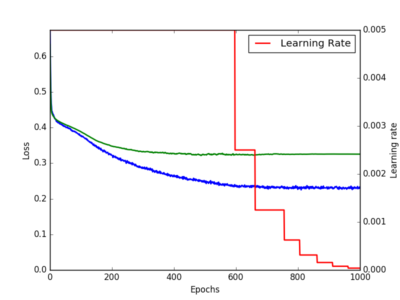
During training the learning rate is reduced when no drop in loss function is observed for 50 epochs. This is conveniently done via the Keras callback ReduceLROnPlateau. The objective to minimize is the binary_crossentropy + the cost from the weight regularization. This makes the reported loss on the train set bigger than the reported loss on the validation set, which can be confusing to see if theres potential overfit. So the binary_crossentropy is also added as an additional metric. This callback from Keras is used at the end of each epoch, and makes it possible to compare the training loss with the validation loss.

#Set network hyper parameters
l1 = 0.000
l2 = 0.016
dropout = 0.5
hidden_dim = 80
#Build neural network
model = Sequential()
model.add(Dropout(0.2, input_shape=(X_train.shape[1],)))
for i in range(3):
 wr = WeightRegularizer(l2 = l2, l1 = l1)
 model.add(Dense(output_dim=hidden_dim, activation="relu", W_regularizer=wr))
 model.add(Dropout(dropout))
wr = WeightRegularizer(l2 = l2, l1 = l1)
model.add(Dense(y_train.shape[1], activation='sigmoid',W_regularizer=wr))
##Compile model and make it ready for optimization
model.compile(loss='binary_crossentropy', optimizer = SGD(lr=0.005, momentum=0.9, nesterov=True), metrics=['binary_crossentropy'])
#Reduce lr callback
reduce_lr = ReduceLROnPlateau(monitor='loss', factor=0.5,patience=50, min_lr=0.00001, verbose=1)
#Training
history = model.fit(X_train, y_train, nb_epoch=1000, batch_size=1000, validation_data=(X_val,y_val), callbacks=[reduce_lr])

Training for 1000 epochs gave a final loss for the trainset of 0.3966 and 0.2330 without the regularization cost.

#Plot Train History
def plot_history(history):
    lw = 2
    fig, ax1 = plt.subplots()
    ax1.plot(history.epoch, history.history['binary_crossentropy'],c='b', label="Train", lw=lw)
    ax1.plot(history.epoch, history.history['val_loss'],c='g', label="Val", lw=lw)
    plt.ylim([0.0, max(history.history['binary_crossentropy'])])
    ax1.set_xlabel('Epochs')
    ax1.set_ylabel('Loss')
    ax2 = ax1.twinx()
    ax2.plot(history.epoch, history.history['lr'],c='r', label="Learning Rate", lw=lw)
    ax2.set_ylabel('Learning rate')
    plt.legend()
    plt.show()
plot_history(history)

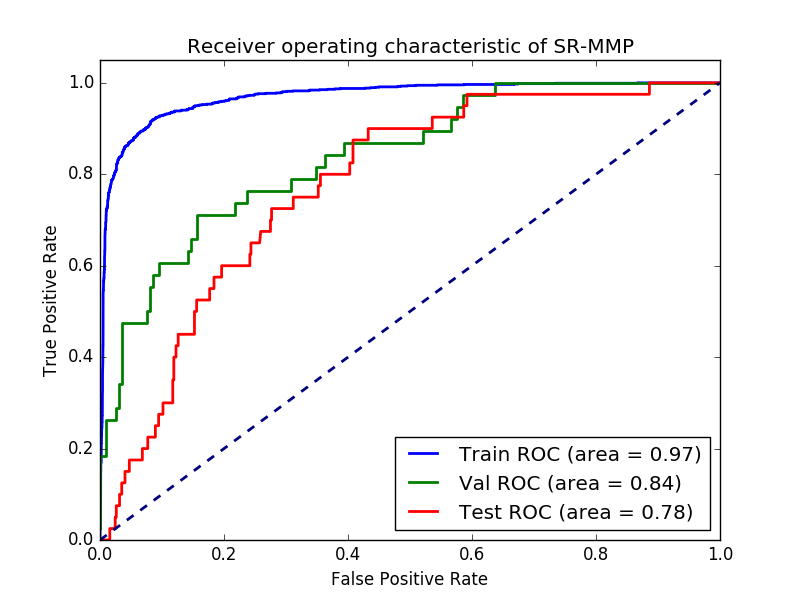
The validation set ended with a loss of 0.3253. For classification task receiver operator charachteristics (ROC) curves and area under the ROC curve are a common way of benchmarking.

def show_auc(model):
    pred_train = model.predict(X_train)
    pred_val = model.predict(X_val)
    pred_test = model.predict(X_test)
    auc_train = roc_auc_score(y_train, pred_train)
    auc_val = roc_auc_score(y_val, pred_val)
    auc_test = roc_auc_score(y_test, pred_test)
    print "AUC, Train:%0.3F Test:%0.3F Val:%0.3F"%(auc_train, auc_test, auc_val)
    fpr_train, tpr_train, _ =roc_curve(y_train, pred_train)
    fpr_val, tpr_val, _ = roc_curve(y_val, pred_val)
    fpr_test, tpr_test, _ = roc_curve(y_test, pred_test)
    plt.figure()
    lw = 2
    plt.plot(fpr_train, tpr_train, color='b',lw=lw, label='Train ROC (area = %0.2f)'%auc_train)
    plt.plot(fpr_val, tpr_val, color='g',lw=lw, label='Val ROC (area = %0.2f)'%auc_val)
    plt.plot(fpr_test, tpr_test, color='r',lw=lw, label='Test ROC (area = %0.2f)'%auc_test)
    plt.plot([0, 1], [0, 1], color='navy', lw=lw, linestyle='--')
    plt.xlim([0.0, 1.0])
    plt.ylim([0.0, 1.05])
    plt.xlabel('False Positive Rate')
    plt.ylabel('True Positive Rate')
    plt.title('Receiver operating characteristic of %s'%prop)
    plt.legend(loc="lower right")
    plt.interactive(True)
    plt.show()
show_auc(model)

So it seems like the model has some predictive power. But how much better is the model than a simple logistic regression with regularization?

#Compare with a Linear model
from sklearn import linear_model
#prepare scoring lists
fitscores = []
predictscores = []
##prepare a log spaced list of alpha values to test
alphas = np.logspace(-2, 4, num=10)
##Iterate through alphas and fit with Ridge Regression
for alpha in alphas:
  estimator = linear_model.LogisticRegression(C = 1/alpha)
  estimator.fit(X_train,y_train)
  fitscores.append(estimator.score(X_train,y_train))
  predictscores.append(estimator.score(X_val,y_val))
#show a plot
import matplotlib.pyplot as plt
ax = plt.gca()
ax.set_xscale('log')
ax.plot(alphas, fitscores,'g')
ax.plot(alphas, predictscores,'b')
plt.xlabel('alpha')
plt.ylabel('Correlation Coefficient')
plt.show()
estimator= linear_model.LogisticRegression(C = 1)
estimator.fit(X_train,y_train)
#Predict the test set
y_pred = estimator.predict(X_test)
print roc_auc_score(y_test, y_pred)

The auc on the test set is 0.63, which is a lot lower than the neural network model. One of the overall best performing algorithms of the Tox21 challenge was a deep neural network. However, they used extra “tricks” such as more neurons, a lot more features in descriptors and fingerprints, and co-modelling of endpoints, as well as careful optimization with cross validation between compound classes found with ECFP4 similarity. Their paper is open access here: doi: 10.3389/fenvs.2015.00080
Please comment and let me know if you find some better regularization or network settings if you try this example, I haven’t done any systematic search and optimization.
Happy modelling
Esben